Tropical Cyclone Intensity Change Prediction Based on Surrounding Environmental Conditions with Deep Learning


1
College of Computer, National University of Defense Technology, Changsha 410073, China
2
College of Meteorology & Oceanography, National University of Defense Technology, Changsha 410073, China
*
Author to whom correspondence should be addressed.
Water 2020, 12(10), 2685; https://doi.org/10.3390/w12102685
Submission received: 4 August 2020
/
Revised: 23 September 2020
/
Accepted: 23 September 2020
/
Published: 25 September 2020
(This article belongs to the Special Issue Hydro-Meteorological Hazards under Climate Change)
Abstract
:Tropical cyclone (TC) motion has an important impact on both human lives and infrastructure. Predicting TC intensity is crucial, especially within the 24 h warning time. TC intensity change prediction can be regarded as a problem of both regression and classification. Statistical forecasting methods based on empirical relationships and traditional numerical prediction methods based on dynamical equations still have difficulty in accurately predicting TC intensity. In this study, a prediction algorithm for TC intensity changes based on deep learning is proposed by exploring the joint spatial features of three-dimensional (3D) environmental conditions that contain the basic variables of the atmosphere and ocean. These features can also be interpreted as fused characteristics of the distributions and interactions of these 3D environmental variables. We adopt a 3D convolutional neural network (3D-CNN) for learning the implicit correlations between the spatial distribution features and TC intensity changes. Image processing technology is also used to enhance the data from a small number of TC samples to generate the training set. Considering the instantaneous 3D status of a TC, we extract deep hybrid features from TC image patterns to predict 24 h intensity changes. Compared to previous studies, the experimental results show that the mean absolute error (MAE) of TC intensity change predictions and the accuracy of the classification as either intensifying or weakening are both significantly improved. The results of combining features of high and low spatial layers confirm that considering the distributions and interactions of 3D environmental variables is conducive to predicting TC intensity changes, thus providing insight into the process of TC evolution.
1. Introduction
Tropical cyclones (TCs) are deep tropical weather systems that occur and develop on the warm ocean surface [1,2]. The disasters TCs can induce, which are among the most destructive natural disasters, are mainly caused by strong winds, heavy rain, and storm surges [3]. TC intensity prediction and rapid intensification (RI) prediction, especially within the warning time of 24 h, remain a major challenge [4]. The difficulty of predicting TC intensity is mainly due to our limited understanding of the complex physical processes and various factors related to TC intensification and decay [5]. Previous studies [6] have concluded that ocean characteristics and internal structural and environmental impacts are the three main factors leading to TC intensity changes. The integration of these factors to gain a further understanding of the TC evolution mechanism holds promise for improving intensity predictions.
Numerous attempts have been made to predict 24 h TC intensity changes using empirical models as well as numerical modelling techniques [7]. In empirical prediction, much of the effort based on statistical–dynamical approaches has gone towards improving TC intensity forecasts via nonlinear approaches using new or optimized predictors [8,9]. Finding and utilizing new predictors that accurately represent TC intensity changes can help to improve the forecasting performance of statistical–dynamical models [7]. For numerical models, different parameterization schemes can be adopted to achieve obvious and unique results in terms of performance and characteristics [10]. Data assimilation can provide the initial conditions for forecasting but does not compensate for the shortcomings of most models. With the development of artificial intelligence, scholars have also attempted to combine machine learning with TC parameters or the outputs of numerical models to forecast TC intensity. Several parameterization theories that represent the direct or feedback effects of a TC itself or the effects of the environment have been exploited. For example, in previous research [4,5], a decision tree model was built using the C4.5 algorithm based on the intensification potential, the intensity changes in the previous 12 h, and zonal wind shear to classify 24 h intensity changes based on the maximum potential intensity (MPI) theory [11]. To better resolve typhoon-induced sea surface temperature cooling (SSTC) feedback in the weather research and forecasting (WRF) model, Jiang et al. [12] applied a nonlinear deep learning algorithm to combine historical data and the target typhoon. This typhoon-induced SSTC feedback acts as negative feedback to modify the storm’s dynamical and thermal structure near the ocean surface through the moisture flux. To generate more accurate intensity predictions, Cloud et al. [13] proposed a feedforward neural network incorporating real-time operational estimation of the current intensity and predictors derived from hurricane weather research and forecasting (HWRF) model forecasts. Machine learning methods can be effectively used for data post-processing and feature learning in relation to the nonlinear processes of TCs.
Air–sea exchange processes control the evolution of TCs [14]. The selection of the predictors and meteorological parameters associated with air–sea interactions is a crucial step in TC prediction. Most TC parameters, which are based on the inner-core dynamics and complex interactions of the TC with the large-scale atmospheric environment and with the underlying ocean, are designed to better predict intensity changes [15,16,17,18]. These parameters also attempt to describe the real TC evolution process as much as possible. However, given the large scale and high complexity of the physical mechanisms of a TC in space, the depiction of TC evolution in terms of these parameters is usually incomplete and circumscribed, which probably accounts for the slow progress in TC intensity prediction [7,12]. In fact, the three-dimensional (3D) environmental field of a TC contains rich features, such as internal circulation, distribution, and interaction [8]. The calculation of TC parameters also utilizes basic environmental variables, including atmospheric and oceanic characteristics, which are closely related to the variations in TC intensity [19]. TCs in different life stages exhibit distinct flow field features [20]. The distribution features and interactions of atmospheric and oceanic variables imply a series of potential changes. In recent years, deep learning has undergone considerable development in the field of computer vision. Convolutional neural networks (CNNs) can extract spatial characteristics from input images by means of simple calculation units that learn features to improve the performance of target detection or classification and do not rely on human intelligence to identify which features are most important [21,22]. Usually, multi-spectral images derived from meteorological satellites leading to a multi-dimensional CNN framework [23]. Two-dimensional convolutional neural networks (2D-CNNs) are commonly used to study translation-invariant features of the input data. Similarly, a three-dimensional convolutional neural network (3D-CNN) can be applied to data samples in the form of 3D cubes [22]. The use of a 3D convolutional kernel provides a simple and effective approach for extracting joint spatial features of TCs that can be used to convert the complex spatial evolution process into simple expressions. Learning the distribution characteristics of spatial environmental variables has become a new approach to estimating TC intensity changes.
To validate our ideas and improve the performance of intensity prediction over a short temporal range of 24 h, we established a deep learning model based on instantaneous joint spatial features to relate the 3D environmental field to TC intensity changes. A 3D-CNN was adopted to extract joint spatial features of 3D environmental variables to estimate 24 h intensity changes, which can also be used to classify TCs as either intensifying or weakening. Experimental results show that compared with previous research, the mean absolute error (MAE) and classification accuracy of the proposed method are competitive and indicate that the capability of TC intensity prediction is improved to some extent.
The remainder of this paper is organized as follows: In Section 2, the data sources as well as the implementation flow and network structure of the method presented in this paper are introduced. In Section 3, we describe the training process and compare the experimental results obtained with multiple methods. Section 4 focuses on further discussion and analysis of the experimental findings. Finally, Section 5 draws some conclusions and presents future prospects.
2. Data and Methodology
2.1. Reanalysis Data and Best Track Data
Reanalysis data provide good conditions for studying the evolution processes of synoptic-scale and mesoscale systems, and they have been widely used in the study of the evolution of TCs [24,25,26]. In this study, the environmental variables considered, including spatial atmospheric data and sea surface data, were obtained from the European Centre for Medium-Range Weather Forecasts (ECMWF) reanalysis data sets (http://apps.ecmwf.int/datasets/data/interim-full-daily/). The spatial resolution is 0.125° × 0.125°, with a temporal resolution of 6 h.
The track data set of TCs that we used is from the Shanghai Typhoon Institute of the China Meteorological Administration (CMA) [27]. This data set includes latitude, longitude, and maximum sustained wind speed (MSW) data recorded every 6 h. Data from the western North Pacific over a period of 22 years (1997–2018) were selected in this study, the distribution of TC samples in this paper is shown in Figure 1. We excluded the samples from narrow sea areas to avoid land-induced disturbances of the TCs [28].
2.2. Outline of Our Methodology
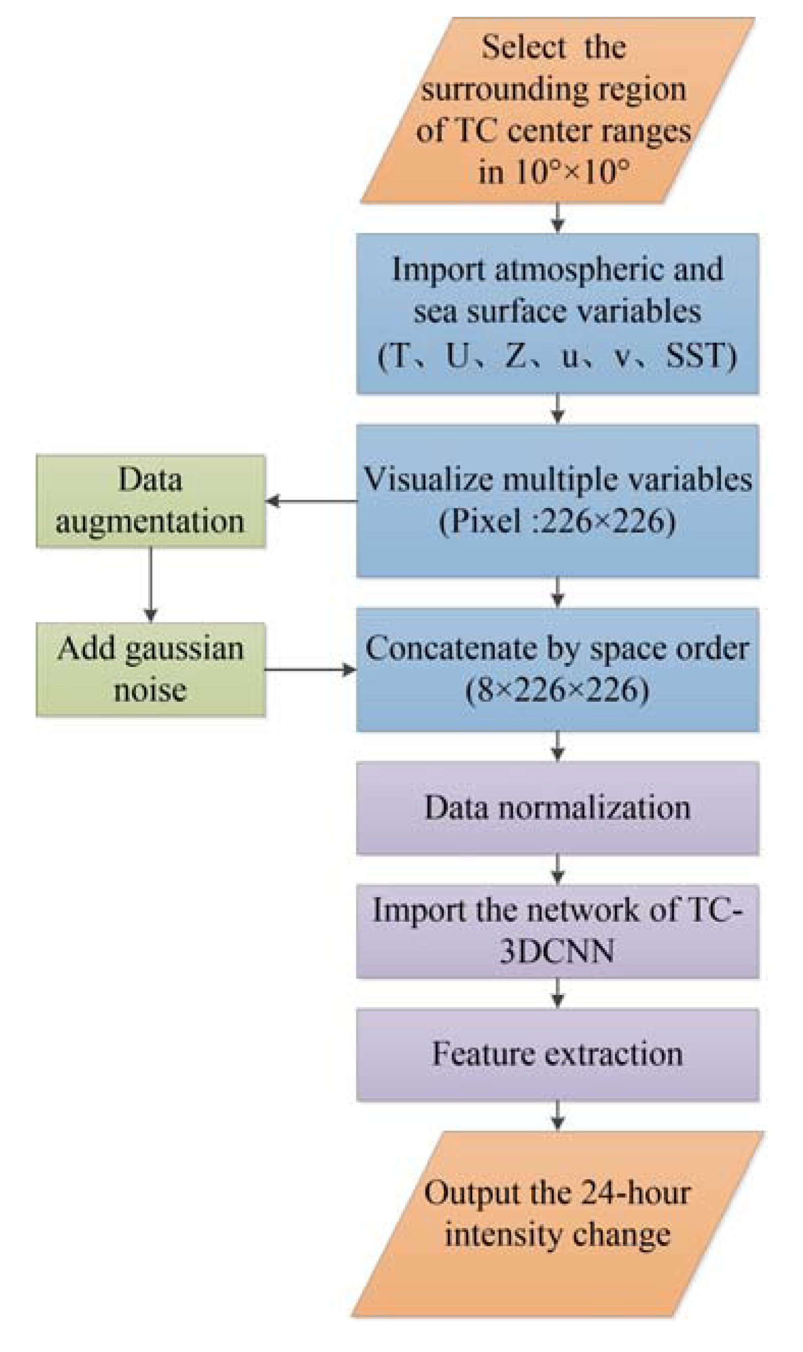
Mature TCs contain macro-structures such as storm eyes, eye walls, and spiral rainbands, which can vary in size from 200 km to 2000 km in diameter and up to 12–16 km in the vertical direction and can extend as far as the tropopause [29]. The overall framework of the intensity change prediction method proposed in this paper is shown in Figure 2, and the proposed prediction algorithm comprises the following steps:
- (1)
- Considering the common and widely used levels in TC studies, we select atmospheric levels of 100, 200, 300, 500, 700, 850, and 1000 hPa that, and utilize environmental variables corresponding to data from the central TC region in a range of 10° × 10° [10].
- (2)
- Previous studies [4,5,16,19] have identified certain meteorological and oceanic characteristics that are closely related to TCs, which can help to inform our work. Thus, we study atmospheric variables including temperature (T), relative humidity (U), wind velocity (u) and (v), and geopotential height (Z). The sea surface temperature (SST) is selected as the sea surface variable.
- (3)
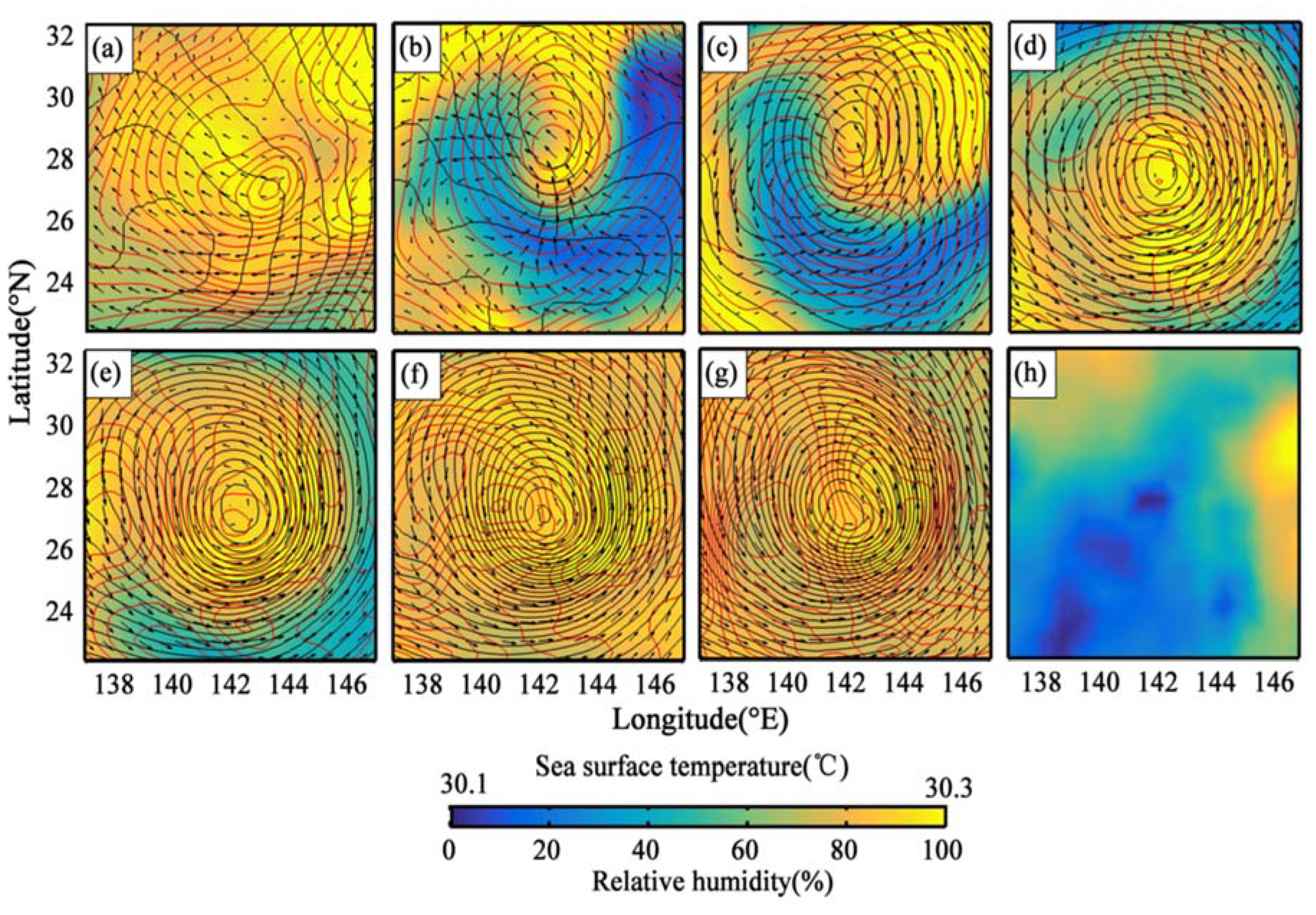
- In general, an image contains detailed features, such as textures, which are defined by continuous spatial changes in the pixels of the image in accordance with certain rules [21,22,30]. Therefore, we visualize multiple variables at various levels in the TC region and specify corresponding representation forms for these variables in images (as shown in Figure 3). In addition, data augmentation is performed to meet the requirements of deep learning in terms of small sample set (see Section 2.3 for details).
- (4)
- The corresponding isobaric surface and sea surface maps of these variables are concatenated in spatial order to form the 3D TC samples. Then, after preprocessing, the samples are input into the model, named TC-3DCNN, and the 24 h intensity changes are finally output. The network structure and feature extraction process are described in detail in Section 2.4.
2.3. Data Augmentation
To meet the requirements of deep learning algorithms, which need a large number of samples for training, data augmentation technology can help enable our subsequent research. Adding noise is a commonly used data augmentation method for image processing in deep learning. Based on the actual noise characteristics of the complex environmental samples, we added Gaussian noise to each original image using a nonlinear distribution with a mean value of = 0 and a variance of . The method of calculating the variance is designed as shown in Equation (1):
where is the maximum value of an image pixel and is the noise effect added to the original image. In this study, we collected a total of 3433 original samples. Each of these samples consisted of 8 images with a pixel resolution of 226 × 226, corresponding to a total of 27,464 images. Among them, 1000 samples were randomly selected as the test set. The remaining 2433 original samples were subjected to data augmentation for model training and validation. Compared with the original image, the addition of noise did not change the sizes of the vector arrows representing the wind information. In addition, the basic features were preserved overall while adding variations in some factors, such as the signal-to-noise ratio. Data augmentation allowed us to increase the number of TC samples available, reducing the time needed to obtain samples manually and avoiding the probability of network over-fitting in the case of insufficient training samples.
2.4. Network Structure Design
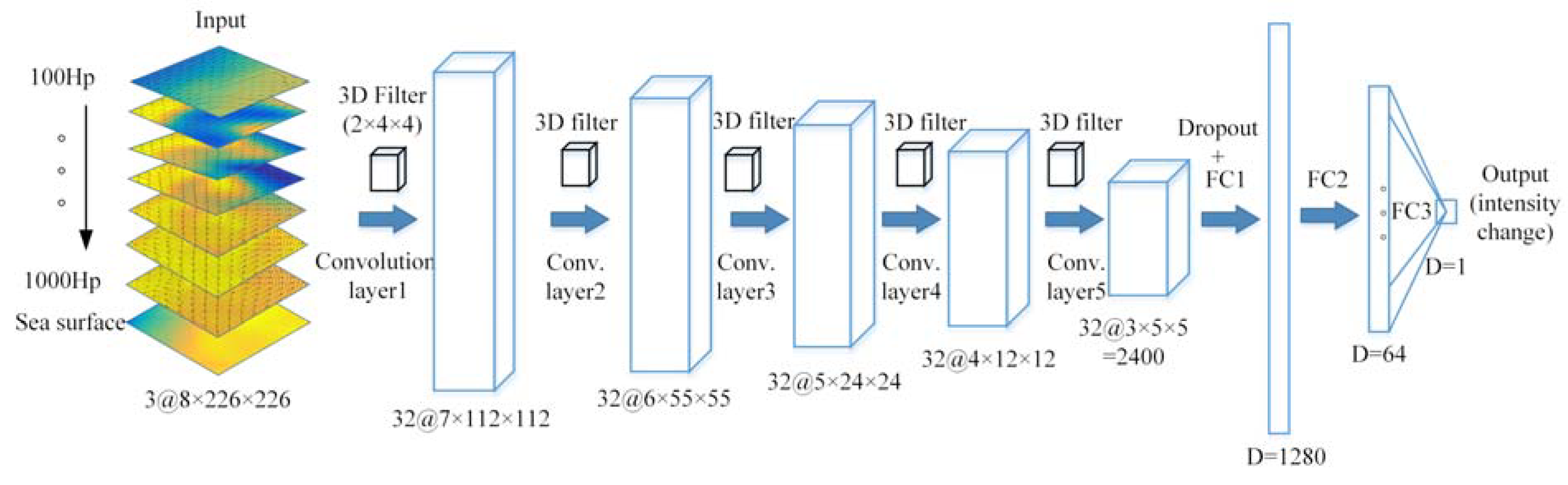
A CNN consists of several processing layers, the purpose of which is to continuously extract abstract features from the input data and match these features with the target under study to perform a regression or classification task [30]. Each layer is composed of numerous neurons, which calculate weighted combinations of the inputs, and the model is trained on a data set to optimize its parameters through the nonlinear action of an activation function. As shown in Figure 4, our TC-3DCNN model is mainly composed of convolutional layers and fully connected (FC) layers; its design is motivated by that of the 2D-CNN called AlexNet [31]. A deeper CNN contains more weights and requires more data to properly adjust these weights. If there are not enough data available, the model can easily be over-fitted. In our work, the number of 3D TC samples available and the different vertical layers prompted us to use a relatively shallow network. The 3D convolution kernels extract information on each input TC from a pixel neighborhood in the spatial center of the cube. After preprocessing, the model had 3 × 8 × 226 × 226 = 1,225,824 (Figure 4) input values. After the five convolutional layers, these features were compressed to 2400 core features. The filter size, number of filters, stride, and other configuration settings are shown in Table 1. For the first convolutional layer, the input array has dimensions of 3 × 8 × 226 × 226, and 32 filters with dimensions of 2 × 4 × 4 are used to extract features with a stride of (1,2,2), transforming the input into 32 × 7 × 112 × 112 = 2,809,856 features. Similarly, the second, third, fourth, and fifth convolutional layers convert the input arrays to 32 × 6 × 55 × 55 = 580,800, 32 × 5 × 26 × 26 = 108,160, 32 × 4 × 12 × 12 = 18,432, and 32 × 3 × 5 × 5 = 2400 features, respectively.
After several convolutional layers, the output from the last convolutional layer is flattened out from a four-dimensional array into a one-dimensional array. The neurons in each FC layer are completely connected to all neurons in the previous layer, and their output can be calculated with a weight and an offset. Finally, the three FC layers were applied to convert the 2400 features into a single predicted 24 h TC intensity change. In this paper, the ReLU function [30] is used as the nonlinear activation function among the layers to study the relationship between the input and output variables, which is very important to effectively mitigate the gradient disappearance problem when training the neural network and is beneficial for gradient descent and error backpropagation. Generally, in CNNs, pooling layers are used to filter out redundant data to reduce the computational complexity. However, the image characteristics of TCs lead us not to use pooling layers because they degrade the resolution of the detected features and cause important characteristics of TCs to be lost [30], such as the contour information. In the TC-3DCNN architecture, we add a dropout layer after the last convolutional layer as a regularization technique to improve the performance of the model [32]. In this layer, during the training process, a certain proportion of the neurons are randomly selected to be disconnected, and only the information transmitted by the remaining neurons is retained to prevent over-fitting of the model. At the end of the learning process, the model calculated the loss function, and the weights were updated through continuous iteration. For the predicted values, we used the mean square error (MSE) as the loss function and the mean absolute error (MAE) as the evaluation standard. The MSE is typically used to detect the deviation between the values predicted by a model and the true values, as defined below:
The MAE is the average of the absolute errors, which can effectively reflect the forecasting error. It is defined as follows:
where N is the number of samples, is a predicted intensity change, and is the corresponding real intensity change.
3. Experiments and Results
3.1. Model Training Process
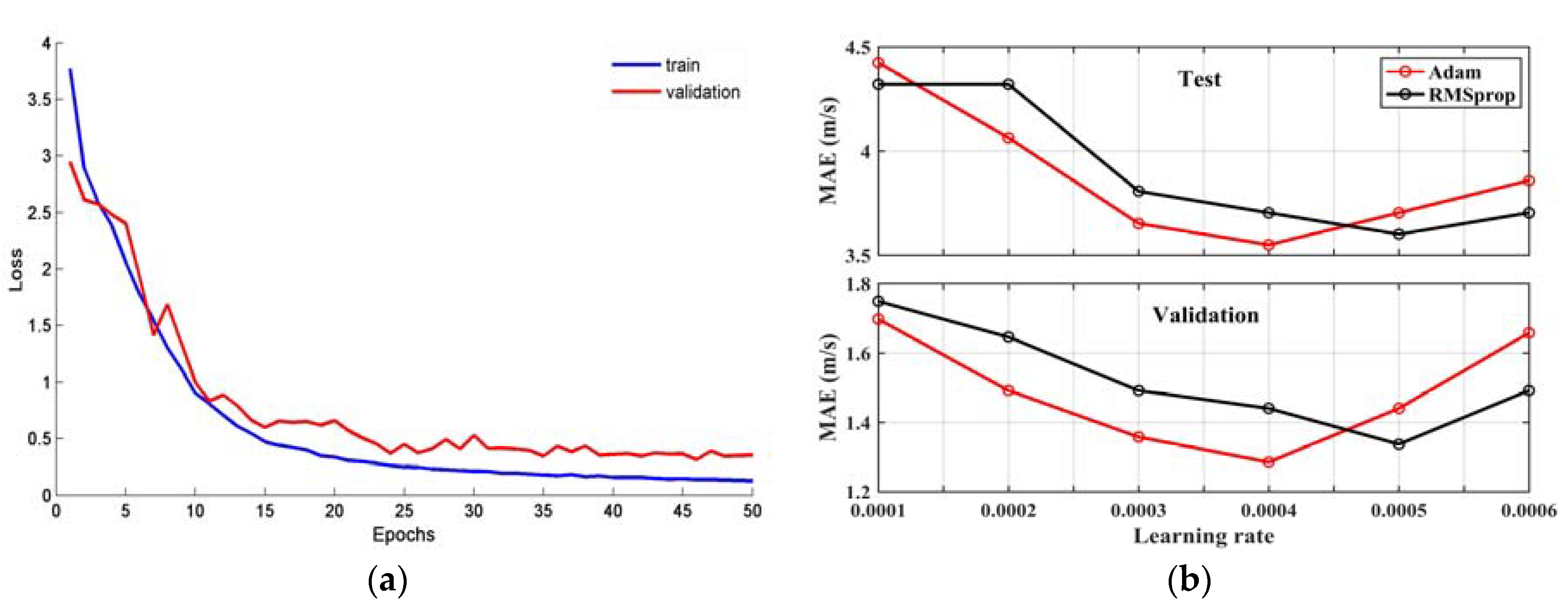
The training for our model starts with the initialization of the weights of the nodes between layers, and the parameters are updated through gradient descent. By iterating over the samples in the training set and minimizing the loss function, the optimal solution is fitted to achieve the optimal performance. To make the model converge better and faster, we normalized the data used in this study. The RGB value of each pixel in each image was divided by the maximum value 255 to normalize the pixels to the range between 0 and 1. The same normalization was applied to the labelled intensity change values. Our model was trained on two Titan Xp GPUs with 12 GB of memory under the Ubuntu 16.04 operating system, and the latest official release of TensorFlow-GPU 2.0 was adopted as the deep learning framework, with Keras as the backend, to build the 3D-CNN. This framework supports CUDA 10.0 and OpenCV 4.3. We performed initial training with different batch sizes to adjust the number of model iterations in each epoch. Since the 3D data consume a large amount of memory, the batch size cannot be too large. However, the loss curves of the model will constantly fluctuate if the batch size is too small, making it difficult to reach convergence. Eventually, we set the batch size to 16 to achieve a stable model training effect. We conducted a relevant experiment over 50 epochs. The learning curves of the model are shown in Figure 5a. The entire training process for our model took approximately 18 min, and the testing process took approximately 5 s.
After the model framework was established, we selected different optimization methods and learning rates to perform relevant experiments. Adaptive moment estimation (Adam) [33,34] is a commonly used optimization and incorporates the advantages of adaptive gradient algorithms to achieve an improved ability to handle non-stationary targets compared to RMSprop [34]; it dynamically adjusts each parameter using the first- and second-order moment estimates of the gradient and updates different parameters through migration correction. The experimental results for the MAE of TC intensity change are shown in Figure 5b when trained at different learning rates using these two optimizations. When the learning rate was 0.0004, our model achieved the best test result of 3.6 m/s. This experiment was repeated 10 times to obtain more accurate estimates of the prediction quality metrics associated with the trained model.
3.2. Feature Importance and Result Analysis
To better understand the feature extraction process for TC intensity change prediction, we studied the importance of the features that affected the performance of the model by varying the information contained in the input images. In our experiment, the contours and wind information were presented on the images in a discrete way, while the relative humidity was a continuous feature presented through color mapping. From the perspective of deep learning, the general rule governing how convolutional layers extract features is that the first convolutional layer mainly extracts rough information such as edges and contours, while the last layer usually extracts subtle features such as the gradients of lines. To investigate the influence of discrete features, we first eliminated all discrete features from the images and retained only the color information, as shown in Figure 6. The resulting images after successive stacking represented the combined spatial features of the relative humidity and SST. As another test condition, we restored the information of the temperature and geopotential height contours, in addition to the color features, and eliminated only the information of the wind vectors, as shown in Figure 7. Using the same network framework and model parameters, the corresponding model performance after training at different learning rates was obtained (see Table 2).
The results in Table 2 indicate that the combined features of the relative humidity, temperature, geopotential height, and SST together endow the model with the best prediction performance for TC intensity changes. The inclusion of the discrete wind vector features has the effect of introducing a certain amount of noise into the model. After their removal, the performance of the model was improved. However, when the temperature and geopotential height contours were also removed, the prediction performance of the model was weakened, implying that the contour information was helpful for allowing the network to learn suitable features for our purposes. Considering the complexity of such multiscale interactions, it is always challenging to improve TC intensity predictions [35]. One possible explanation is that the distributions and interactions between the isotherms and geopotential height contours reflect the spatial impact of cold and warm advection on the trough system [36]. The interaction between a TC and such a trough can result in various changes, from RI to rapid weakening in the TC [35]. The presence of a trough in the upper troposphere can give rise to unique forces affecting convection and TC intensification [37]. Such troughs are also associated with adverse environmental conditions, such as increased vertical wind shear. Previous studies [38] have also shown that one potential pathway by which an upper-tropospheric trough can induce TC intensification involves the trough acting as a source of angular momentum in the TC outflow layer. The convergence of the fluxes of angular momentum can enhance the secondary circulation of the TC, with a stronger upper-tropospheric outflow favoring rising motion in the inner core, greater convective activity, and TC intensification [35,39].
The findings also demonstrate that the joint spatial features of relative humidity and SST in the images provide important information for the prediction of intensity changes. The relative humidity and SST are usually considered as the main thermal factors affecting TC intensity changes, with a higher relative humidity providing the favourable conditions of humidity and water vapor for TC intensification, while the underlying ocean surface is the main source of energy for TC development. A higher SST is generally more conducive to TC intensification, but there is no direct linear relationship between the SST and TC intensification. The main reason for this phenomenon is that an excessively high SST will lead to excessive warming at the top of the TC, causing the gas column where the warm core is located to tend towards stability, and thus inhibiting TC development [40]. Our deep neural network extracts the joint spatial features of TC variables from the 3D perspective to gain insight into intensity changes, providing an effective means of addressing the complexity of fusing multiple factors related to TC intensity change prediction.
After the removal of the discrete wind vectors from the images containing all environmental variables, the model yielded the minimum forecasting errors. The corresponding results were also the most robust, demonstrating the excellent performance of our model under these conditions. A scatterplot of the actual and predicted values for the 1000 test samples, with a correlation coefficient of 0.76 shown in Figure 8a. The values of the TC intensity changes are mainly concentrated near the middle of the regression line, whereas the forecast points near the upper and lower ends of the regression line show large deviations. Figure 8b shows the detailed forecasting errors of the samples for different intensity change values, ranging from the strongest decreases in intensity to the strongest increases in intensity. The prediction errors are larger near the extreme values of intensity change. In addition, the model predictions are likely to be overestimated for samples with weakening intensity, while for samples with increasing intensity, the model tends to underestimate. These findings indicate that a small number of TCs that rapidly weakened or intensified led to relatively large prediction errors of the model. The instability caused by such dramatic changes in TC intensity, in contrast to the relatively steady evolution characteristics of most TCs in the prediction window, makes the prediction task more complex and difficult. On the other hand, we have made statistics of different categories of TC intensity, as shown in Table 3. From the results, the extremely strong TCs make it more difficult to predict intensity change. The reason may be that the more severe TC is, the more complex the atmospheric dynamics process will be. At this time, the prediction of TC intensity after 24 h that only based on the 3D distribution of the environmental variables at the current moment will produce a large error. In this case, it is necessary to improve the prediction skills to improve the prediction performance of the model.
3.3. Model Performance Evaluation
We compared our results with those of other methods, including a traditional statistical model and a widely used numerical model. Based on the current intensity of a TC, intensity change prediction can be realized in combination with the prediction of the intensity 24 h in the future, and the MAEs of these two predictions are numerically equivalent. As the statistical and numerical forecasting models considered for comparison, we selected the Western North Pacific Tropical Cyclone Intensity Prediction Scheme (WIPS) and the Tropical Cyclone Model based on the Global/Regional Assimilation and Prediction System (GRAPES-TCM) [10], respectively. The average intensity errors over the past five years from CMA and National Hurricane Center (NHC) reports were used for the comparison. The results, which are shown in Table 4, suggest that the MAE of our model is better than those of the existing models. The MAE of our model is 4.1 m/s, while the MAEs of the statistical and numerical models for the test period of 2012–2016 are 5.6 m/s and 7.0 m/s, respectively. Thus, we achieved competitive experimental results by considering only the current 3D status of the TC, which demonstrates the high learning efficiency of a 3D-CNN for this problem and also proves that our method successfully captures the implicit patterns relating the distributions of the environmental variables to TC variations.
The samples can be assigned three different category labels: positive (indicating an increase in intensity), negative (indicating a decrease in intensity), and zero (indicating no change in intensity). Thus, in addition to their numerical magnitudes, the prediction results were also evaluated in terms of the category to which each sample belonged. Our model could quickly predict the categories of the samples. The prediction results for the three categories were calculated. The MAE for intensifying samples was 3.1 m/s, the MAE for weakening samples was 4.6 m/s, and for samples showing no change in intensity, the MAE was 2.4 m/s. These findings demonstrate that the model was less sensitive for negative samples. The reason might be that the training set contained relatively few negative samples, leading to an imbalance among the categories. In real applications, the intensification of a TC is usually more valuable to predict [4,5] because this enables early warning before severe damage, which is beneficial for prevention and risk avoidance. For category classification, we used the Accuracy as a reliable indicator for model evaluation. The formula is as follows:
In this formula, TP represents the true positive classifications, TN is the number of true negative classifications, FP is the number of false positive classifications (weakening TCs classified as intensifying), and FN corresponds to the number of false negative classifications (intensifying TCs classified as weakening). For fair comparison, the same operation was performed on the basis of the classification criteria specified in the related reference [4]. The results are listed in Table 5. For strong intensity increases ( (m/s)/24 h) and decreases ( (m/s)/24 h), the classification accuracy is 96.1%. For moderate intensification ( (m/s)/24 h) and weakening ( (m/s)/24 h), the classification accuracy is 92.0%. For TCs ( (m/s)/24 h) and ( (m/s)/24 h), the classification accuracy is 83.1%. The results suggest that compared with the results reported in reference [5] based on the decision tree method, our deep learning approach offers better classification accuracy and more stable performance under different criteria for intensity change classification.
4. Discussion
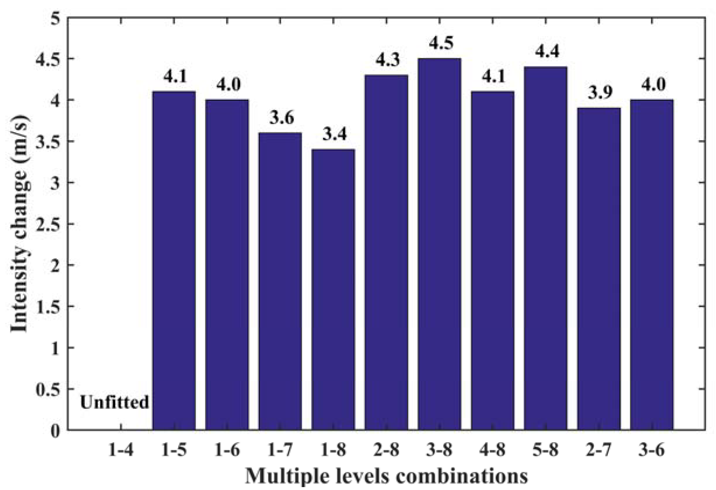
The impact of each part of the 3D spatial structure of a TC on the TC intensity change prediction was studied by considering different combinations of levels. The histogram in Figure 9 shows the prediction errors under different combinations of multiple levels, from which it can be seen that the MAE for the combination of all levels (1–8) was the smallest, thus proving the excellent performance of the TC-3DCNN model and the necessity and rationality of considering this spatial combination. We studied different combinations layer by layer, from the top down and from the bottom up. For the 1–7 combination, the MAE difference relative to the 1–8 combination was 0.2 m/s, indicating that the sea surface variable had a small positive effect on TC intensity change prediction in this study. Between the 2–8 and 1–8 combinations, the MAE difference was 0.9 m/s, proving that the top layer (100 hPa) had a larger positive impact on the model than the sea surface layer, with a higher contribution in terms of error reduction. To a certain extent, this finding demonstrates that on average, the contribution of the characteristics at 100 hPa to the overall intensity change is greater than that of the sea surface characteristics. This difference can probably be attributed to the fact that the temperature, which offers relatively little useful information, was the only sea surface variable considered in this experiment. It might also be that the high–low spatial circulation and distribution characteristics of multiple environmental variables are more relevant to the trend of TC intensity change than any single variable (such as the SST). Compared with the 1–7 combination, the removal of the 1000 hPa isobaric surface (corresponding to the 1–6 combination) led to an increase of 0.4 m/s in the MAE value. There was no obvious difference between the 1–6 and 1–5 combinations. With the continuous removal of lower layers, it eventually became impossible for the model to converge for the 1–4 combination. It should be noted that in this analysis, it is meaningful only to consider the relative contribution of each layer in comparison with the adjacent combination. The change in the MAE value caused by the inclusion or exclusion of each layer is not a simple linear addition or subtraction because the 3D characteristics of the different combinations are composite in nature. If one layer of the combination changes, so do its overall features. Therefore, the impact and contribution of each layer will also change between different combinations. For example, the MAE value of the 2–7 combination was increased by 0.5 m/s compared with that of the 1–8 combination, indicating that the common contribution of the 100 hPa and sea surface layers under this condition was 0.5 m/s. However, this value is not equal to the simple sum of the sea surface (0.2 m/s) and 100 hPa (0.9 m/s) contributions. From the above experiments, we can see that the contribution of each layer to the prediction of the intensity change is different, and the mixed distributions of the features at high levels tend to show a more prominent prediction effect than those at low levels. Nevertheless, the combination of all high and low layers yields the best prediction results, confirming that considering the distributions and interactions of 3D environmental variables is helpful for predicting TC intensity changes.
In addition to the above results, we also explored the differences between the original data and TC images and the impact of data augmentation on the performance of our network. Using the same model architecture and configuration parameters, we randomly selected 1000 of the original samples as the test set and constructed three different training sets: the original samples with no data augmentation, the training set obtained by applying data augmentation to half of the original samples, and the training set obtained by applying data augmentation to all of the original samples. The test results for the experiment are shown in Table 6.
It can be intuitively seen from the comparison in Table 6 that our deep learning model is more efficient for processing the data of image patterns. In this paper, the distribution of the contours and their implicit interactions with the weather systems are the potential learning features. In addition, the thermal effects of sea surface temperature and relative humidity are also important factors to improve the prediction performance of the model. The mixed characteristics of these variables are the key to model predictions. In addition, the visual features of the images also contribute to the understanding and interpretation of variables, which is what we focus on next. On the other hand, training the network on samples subjected to data augmentation led to lower prediction errors and higher classification accuracy, thus directly demonstrating the data augmentation technique can be successfully applied for the prediction of TC intensity changes. Data augmentation simultaneously accelerates the convergence speed of the model and improves its performance.
5. Conclusion and Prospects
In this study, we hypothesized that joint spatial features of 3D environmental variables should be valuable indicators for predicting TC evolution that are correlated with TC intensity changes. To explore this idea, we took advantage of 22 years of environmental data made available by ECMWF and trained a deep learning model to predict and classify TC intensity changes. The proposed prediction method is solely based on the visual patterns of TC environmental variables as represented in images and does not require any calculation of TC parameters. The other innovation of the proposed method lies in data augmentation based on a small number of accurate TC samples, which enabled us to solve the problem of an insufficient number of samples for deep learning. Through data augmentation, we were able to better optimize our model and improve its training efficiency.
Comparisons of the statistical results showed that our deep neural network could successfully forecast TC intensity changes. However, the prediction performance of the model was found to suffer for TCs that rapidly weaken or intensify. We also studied the influence of each part of the 3D spatial structure of a TC on TC intensity change prediction by considering different combinations of levels and simulated instantaneous 3D TC states to better represent the mixed spatial features. The contribution of each layer to intensity change prediction was found to be different for different layer combinations and did not follow simple linear addition or subtraction rules. The results achieved with the full combination of high and low layers confirmed that considering the distributions and interactions of 3D environmental variables is helpful in predicting TC intensity changes. The implicit patterns relating the joint spatial features to TC intensity changes were successfully captured and learned by our model.
The proposed method can be further optimized. For example, the fine feature and its range associated with TC intensity change are still worth studying. We believe that addressing these issues will enable further enhancement of the forecasting accuracy. In the future, we can continue to study these issues and extract additional fused features to enable prediction over longer time horizons and for other TC attributes of concern, such as life span. Furthermore, we can apply this method to the study of different sea regions and landfall TCs. Finally, the RI patterns of TCs will be an interesting and significant topic of research.
Author Contributions
X.W. and W.W. conceived and designed the experiments; X.W. performed the experiments and wrote the paper; and W.W., B.Y., and X.W. assisted with field work, discussion, and revisions. All authors have read and agreed to the published version of the manuscript.
Funding
This research was funded by the National Science Foundation of China (61972411).
Acknowledgments
All the data used in this study are available as follows: (1) The environmental variables are available from the European Centre for Medium-Range Weather Forecasts reanalysis data sets (http://apps.ecmwf.int/data-sets/data/interim-full-daily/). (2) The best track data set for TCs is provided by the Shanghai Typhoon Institute of the China Meteorological Administration (http://www.typhoon.gov.cn/).
Conflicts of Interest
The authors declare no conflict of interest.
References
- Gao, S.; Wang, D.; Hong, H.; Wu, N.; Li, T. Evaluation of Warm-Core Structure in Reanalysis and Satellite Data Sets Using HS3 Dropsonde Observations: A Case Study of Hurricane Edouard (2014). J. Geophys. Res. Atmos. 2018, 123, 6713–6731. [Google Scholar] [CrossRef]
- Fink, A.H.; Speth, P. Tropical cyclones. Naturwissenschaften 1998, 85, 482–493. [Google Scholar] [CrossRef]
- Zhang, Q.; Wu, L.; Liu, Q. Tropical Cyclone Damages in China 1983–2006. Bull. Am. Meteorol. Soc. 2009, 90, 489–496. [Google Scholar] [CrossRef] [Green Version]
- Gao, S.; Zhang, W.; Liu, J.; Lin, I.I.; Chiu, L.S.; Cao, K. Improvements in Typhoon Intensity Change Classification by Incorporating an Ocean Coupling Potential Intensity Index into Decision Trees*,+. Weather Forecast. 2016, 31, 95–106. [Google Scholar] [CrossRef]
- Zhang, W.; Gao, S.; Chen, B.; Cao, K. The application of decision tree to intensity change classification of tropical cyclones in western North Pacific. Geophys. Res. Lett. 2013, 40, 1883–1887. [Google Scholar] [CrossRef]
- Russell, L.E.; Lianshou, C.; Jim, D.; Robert, R.; Yuqing, W.; Liguang, W. Advances in Understanding and Forecasting Rapidly Changing Phenomena in Tropical Cyclones. Trop. Cyclone Res. Rev. 2013, 2, 13–24. [Google Scholar] [CrossRef]
- Lee, W.; Kim, S.-H.; Chu, P.; Moon, I.-J.; Soloviev, A.V. An Index to Better Estimate Tropical Cyclone Intensity Change in the Western North Pacific. Geophys. Res. Lett. 2019, 46, 8960–8968. [Google Scholar] [CrossRef] [Green Version]
- Kaplan, J.; Rozoff, C.M.; DeMaria, M.; Sampson, C.R.; Kossin, J.P.; Velden, C.S.; Cione, J.J.; Dunion, J.; Knaff, J.A.; Zhang, J.A.; et al. Evaluating Environmental Impacts on Tropical Cyclone Rapid Intensification Predictability Utilizing Statistical Models. Weather Forecast. 2015, 30, 1374–1396. [Google Scholar] [CrossRef]
- Balaguru, K.; Foltz, G.R.; Leung, L.R.; Hagos, S.; Judi, D.R. On the Use of Ocean Dynamic Temperature for Hurricane Intensity Forecasting. Weather Forecast. 2018, 33, 411–418. [Google Scholar] [CrossRef]
- Chen, R.; Wang, X.; Zhang, W.; Zhu, X.; Li, A.; Yang, C. A hybrid CNN-LSTM model for typhoon formation forecasting. GeoInformatica 2019, 23, 375–396. [Google Scholar] [CrossRef]
- Makarieva, A.M.; Gorshkov, V.G.; Nefiodov, A.V.; Chikunov, A.V.; Sheil, D.; Nobre, A.D.; Nobre, P.; Li, B.-L. Hurricane’s maximum potential intensity and surface heat fluxes. arXiv 2018, arXiv:1810.12451. [Google Scholar]
- Jiang, G.Q.; Xu, J.; Wei, J. A Deep Learning Algorithm of Neural Network for the Parameterization of Typhoon-Ocean Feedback in Typhoon Forecast Models. Geophys. Res. Lett. 2018, 45, 3706–3716. [Google Scholar] [CrossRef] [Green Version]
- Cloud, K.A.; Reich, B.J.; Rozoff, C.M.; Alessandrini, S.; Lewis, W.E.; Monache, L.D. A Feed Forward Neural Network Based on Model Output Statistics for Short-Term Hurricane Intensity Prediction. Weather Forecast. 2019, 34, 985–997. [Google Scholar] [CrossRef]
- Emanuel, K. A Similarity Hypothesis for Air–Sea Exchange at Extreme Wind Speeds. J. Atmos. Sci. 2003, 60, 1420–1428. [Google Scholar] [CrossRef]
- Ito, K.; Kuroda, T.; Saito, K.; Wada, A. Forecasting a Large Number of Tropical Cyclone Intensities around Japan Using a High-Resolution Atmosphere–Ocean Coupled Model. Weather Forecast. 2015, 30, 793–808. [Google Scholar] [CrossRef]
- Zhang, M.; Zhou, L.; Chen, D.; Wang, C. A genesis potential index for Western North Pacific tropical cyclones by using oceanic parameters. J. Geophys. Res. Oceans 2016, 121, 7176–7191. [Google Scholar] [CrossRef] [Green Version]
- Sitkowski, M.; Kossin, J.P.; Rozoff, C.M. Intensity and Structure Changes during Hurricane Eyewall Replacement Cycles. Mon. Weather Rev. 2011, 139, 3829–3847. [Google Scholar] [CrossRef]
- Ge, X.; Li, T.; Peng, M. Effects of Vertical Shears and Midlevel Dry Air on Tropical Cyclone Developments*. J. Atmos. Sci. 2013, 70, 3859–3875. [Google Scholar] [CrossRef]
- Wijnands, J.S.; Qian, G.; Kuleshov, Y. Variable Selection for Tropical Cyclogenesis Predictive Modeling. Mon. Weather Rev. 2016, 144, 4605–4619. [Google Scholar] [CrossRef]
- Ge, K.; Colle, B.A. Multidecadal Historical Trends in Tropical Cyclone Intensity and Evolution Characteristics for Two North Atlantic Subbasins. J. Geophys. Res. Atmos. 2019, 124, 9893–9904. [Google Scholar] [CrossRef]
- Han, Y.; Gao, Y.; Zhang, Y.; Wang, J.; Yang, S. Hyperspectral Sea Ice Image Classification Based on the Spectral-Spatial-Joint Feature with Deep Learning. Remote Sens. 2019, 11, 2170. [Google Scholar] [CrossRef] [Green Version]
- Li, Y.; Zhang, H.; Shen, Q. Spectral–Spatial Classification of Hyperspectral Imagery with 3D Convolutional Neural Network. Remote Sens. 2017, 9, 67. [Google Scholar] [CrossRef] [Green Version]
- Lee, J.; Im, J.; Cha, D.; Park, H.; Sim, S. Tropical Cyclone Intensity Estimation Using Multi-Dimensional Convolutional Neural Networks from Geostationary Satellite Data. Remote Sens. 2019, 12, 108. [Google Scholar] [CrossRef] [Green Version]
- Maloney, E.D.; Hartmann, D.L. Modulation of Eastern North Pacific Hurricanes by the Madden–Julian Oscillation. J. Clim. 2000, 13, 1451–1460. [Google Scholar] [CrossRef]
- Schenkel, B.A.; Hart, R.E. An Examination of Tropical Cyclone Position, Intensity, and Intensity Life Cycle within Atmospheric Reanalysis Datasets. J. Clim. 2012, 25, 3453–3475. [Google Scholar] [CrossRef]
- Cocks, S.B.; Gray, W.M. Variability of the Outer Wind Profiles of Western North Pacific Typhoons: Classifications and Techniques for Analysis and Forecasting. Mon. Weather Rev. 2002, 130, 1989–2005. [Google Scholar] [CrossRef] [Green Version]
- Ying, M.; Zhang, W.; Yu, H.; Lu, X.; Feng, J.; Fan, Y.; Zhu, Y.; Chen, D. An Overview of the China Meteorological Administration Tropical Cyclone Database. J. Atmos. Ocean. Technol. 2014, 31, 287–301. [Google Scholar] [CrossRef] [Green Version]
- Zhang, W.; Leung, Y.; Wang, Y. Cluster analysis of post-landfall tracks of landfalling tropical cyclones over China. Clim. Dyn. 2012, 40, 1237–1255. [Google Scholar] [CrossRef]
- Kerns, B.W.; Chen, S.S. Cloud Clusters and Tropical Cyclogenesis: Developing and Nondeveloping Systems and Their Large-Scale Environment. Mon. Weather Rev. 2013, 141, 192–210. [Google Scholar] [CrossRef] [Green Version]
- Chen, B.-F.; Chen, B.; Lin, H.-T.; Elsberry, R.L. Estimating Tropical Cyclone Intensity by Satellite Imagery Utilizing Convolutional Neural Networks. Weather Forecast. 2019, 34, 447–465. [Google Scholar] [CrossRef]
- Krizhevsky, A.; Sutskever, I.; Hinton, G.E. ImageNet Classification with Deep Convolutional Neural Networks. Commun. ACM 2017, 60, 84–90. [Google Scholar] [CrossRef]
- Srivastava, N.; Hinton, G.; Krizhevsky, A.; Sutskever, I.; Salakhutdinov, R. Dropout: A Simple Way to Prevent Neural Networks from Overfitting. J. Mach. Learn. Res. 2014, 15, 1929–1958. [Google Scholar]
- Nair, V.; Hinton, G.E. Rectified linear units improve Restricted Boltzmann machines. In Proceedings of the 27th International Conference on Machine Learning, ICML 2010, Haifa, Israel, 21–25 June 2010; pp. 807–814. [Google Scholar]
- Kingma, D.P.; Ba, J. Adam: A Method for Stochastic Optimization. In Proceedings of the 3rd International Conference for Learning Representations, San Diego, CA, USA, 7–9 May 2014. [Google Scholar]
- Fischer, M.S.; Tang, B.H.; Corbosiero, K.L. A Climatological Analysis of Tropical Cyclone Rapid Intensification in Environments of Upper-Tropospheric Troughs. Mon. Weather Rev. 2019, 147, 3693–3719. [Google Scholar] [CrossRef]
- Shishi Liu, S.L. Atmospheric Dynamics; Peking University Press: Beijing, China, 1991; p. 536. [Google Scholar]
- Fischer, M.S.; Tang, B.H.; Corbosiero, K.L. Assessing the Influence of Upper-Tropospheric Troughs on Tropical Cyclone Intensification Rates after Genesis. Mon. Weather Rev. 2017, 145, 1295–1313. [Google Scholar] [CrossRef] [Green Version]
- Molinari, J.; Vollaro, D. External Influences on Hurricane Intensity. Part I: Outflow Layer Eddy Angular Momentum Fluxes. J. Atmos. Sci. 1989, 46, 1093–1105. [Google Scholar] [CrossRef] [Green Version]
- Kaplan, J.; DeMaria, M. Large-Scale Characteristics of Rapidly Intensifying Tropical Cyclones in the North Atlantic Basin. Weather Forecast. 2003, 18, 1093–1108. [Google Scholar] [CrossRef] [Green Version]
- Chan, J.; Duan, Y.; Shay, L.K. Tropical Cyclone Intensity Change from a Simple Ocean–Atmosphere Coupled Model. J. Atmos. Sci. 2001, 58, 154–172. [Google Scholar] [CrossRef]
Figure 1.
Distribution of tropical cyclones (red points).

Figure 2.
Flow chart of tropical cyclone (TC) intensity change prediction.

Figure 3.
Images of atmospheric and oceanic variables at each level: (a) 100 hPa, (b) 200 hPa, (c) 300 hPa, (d) 500 hPa, (e) 700 hPa, (f) 850 hPa, (g) 1000 hPa, and (h) sea surface. In each image, vector arrows represent wind information (length for magnitude (m/s), arrowhead for direction), red contours represent temperature (°C), black contours represent geopotential height (gpm), and colors represent relative humidity (%) in (a–g) and sea surface temperature (SST) (°C) in (h). The time corresponding to the depicted TC state is 06:00 a.m. on 31 August 2017.

Figure 4.
Flow chart and architecture of the TC-3DCNN (three-dimensional convolutional neural network) model.
Figure 4.
Flow chart and architecture of the TC-3DCNN (three-dimensional convolutional neural network) model.

Figure 5.
(a) Model learning curves: training loss (blue line) and validation loss (red line). (b) Model testing and validation results when optimized with Adam (red line) and RMSprop (black line) at different learning rates.
Figure 5.
(a) Model learning curves: training loss (blue line) and validation loss (red line). (b) Model testing and validation results when optimized with Adam (red line) and RMSprop (black line) at different learning rates.

Figure 6.
Images of atmospheric and oceanic variables at each level: (a) 100 hPa, (b) 200 hPa, (c) 300 hPa, (d) 500 hPa, (e) 700 hPa, (f) 850 hPa, (g) 1000 hPa, and (h) sea surface. In each image, the colors in (a–g) represent relative humidity (%), and those in (h) represent the SST (°C).
Figure 6.
Images of atmospheric and oceanic variables at each level: (a) 100 hPa, (b) 200 hPa, (c) 300 hPa, (d) 500 hPa, (e) 700 hPa, (f) 850 hPa, (g) 1000 hPa, and (h) sea surface. In each image, the colors in (a–g) represent relative humidity (%), and those in (h) represent the SST (°C).

Figure 7.
Images of atmospheric and oceanic variables at each level: (a) 100 hPa, (b) 200 hPa, (c) 300 hPa, (d) 500 hPa, (e) 700 hPa, (f) 850 hPa, (g) 1000 hPa, and (h) sea surface. In each image, red contours represent temperature (°C), black contours represent geopotential height (gpm), and colors represent relative humidity (%) in (a–g) and SST (°C) in (h).

Figure 8.
(a) Scatterplot of TC-3DCNN forecasting results. The least squares regression line (black line), correlation coefficient R, and MAE are also shown. (b) Forecasting error distribution with respect to TC intensity change.
Figure 8.
(a) Scatterplot of TC-3DCNN forecasting results. The least squares regression line (black line), correlation coefficient R, and MAE are also shown. (b) Forecasting error distribution with respect to TC intensity change.

Figure 9.
Performance comparison of multi-level combinations of TC variables: 1–8 = 100 hPa-sea surface, 1–7 = 100–1000 hPa, 1–6 = 100–850 hPa, 1–5 = 100–700 hPa, 1–4 = 100–500 hPa, 2–8 = 200 hPa-sea surface, 3–8 = 300 hPa-sea surface, 4–8 = 500 hPa-sea surface, 5–8 = 500 hPa-sea surface, 2–7 = 200–1000 hPa, and 3–6 = 300–850 hPa.


Table 1.
Model architecture of TC-3DCNN (including five convolutional layers and three fully connected (FC) layers).
Table 1.
Model architecture of TC-3DCNN (including five convolutional layers and three fully connected (FC) layers).
| Layer | Input Shape | Filter Size | Stride | Activation | Output Shape |
|---|---|---|---|---|---|
| Conv3D.1 | 3 × 8 × 226 × 226 | 32 × 2 × 4 × 4 | (1,2,2) | ReLU | 32 × 7 × 112 × 112 |
| Conv3D.2 | 32 × 7 × 112 × 112 | 32 × 2 × 4 × 4 | (1,2,2) | ReLU | 32 × 6 × 55 × 55 |
| Conv3D.3 | 32 × 6 × 55 × 55 | 32 × 2 × 4 × 4 | (1,2,2) | ReLU | 32 × 5 × 26 × 26 |
| Conv3D.4 | 32 × 5 × 26 × 26 | 32 × 2 × 4 × 4 | (1,2,2) | ReLU | 32 × 4 × 12 × 12 |
| Conv3D.5 | 32 × 4 × 12 × 12 | 32 × 2 × 4 × 4 | (1,2,2) | ReLU | 32 × 3 × 5 × 5 |
| Dropout | 32 × 3 × 5 × 5 | — | — | — | 32 × 3 × 5 × 5 |
| FC1 | 2400 | — | — | ReLU | 1280 |
| FC2 | 1280 | — | — | ReLU | 64 |
| FC3 | 64 | — | — | Tanh | 1 |
Table 2.
Mean absolute errors (MAEs) (m/s) of the models trained on the three combinations of variables at different learning rates.
Table 2.
Mean absolute errors (MAEs) (m/s) of the models trained on the three combinations of variables at different learning rates.
| Combination | 0.0001 | 0.0002 | 0.0003 | 0.0004 | 0.0005 | 0.0006 |
|---|---|---|---|---|---|---|
| U, T, Z, u, v, SST | 4.4 | 4.1 | 3.7 | 3.6 | 3.7 | 3.9 |
| U, SST | 4.3 | 4.1 | 3.7 | 3.7 | 3.8 | 3.9 |
| U, T, Z, SST | 4.1 | 3.9 | 3.4 | 3.4 | 3.7 | 3.8 |
Table 3.
The MAE (m/s) in the different categories of TC intensity (m/s).
| Category | TC Intensity | MAE |
|---|---|---|
| Tropical depression | 9–17 | 3.0 |
| Tropical storm | 17–32 | 3.5 |
| Typhoon | 32–43 | 3.2 |
| Severe typhoon | 43–54 | 3.5 |
| Super typhoon | ≥54 | 3.9 |
Table 4.
Comparison with existing models in terms of the MAE (m/s) of TC intensity change prediction
Table 4.
Comparison with existing models in terms of the MAE (m/s) of TC intensity change prediction
| Model | Test Period | Sample Size | MAE |
|---|---|---|---|
| WIPS | 2012–2016 | - | 5.6 |
| GRAPES-TCM | 2012–2016 | - | 7.0 |
| TC-3DCNN | 2012–2016 | 200 | 4.1 |
Table 5.
Comparison of classification accuracy under different classification criteria
| Classification Criteria (m/s)/24 h | Decision Tree | TC-3DCNN | ||
|---|---|---|---|---|
| Sample Size | Accuracy | Sample Size | Accuracy | |
| and | 693 | 90.2% | 408 | 94.9% |
| and | 1024 | 81.5% | 769 | 91.5% |
| and | 1246 | 77.4% | 1000 | 83.0% |
Table 6.
Performance evaluation with different data augmentation ratios (the different accuracy metrics correspond to the three sets of classification criteria in Table 4).
Table 6.
Performance evaluation with different data augmentation ratios (the different accuracy metrics correspond to the three sets of classification criteria in Table 4).
| Ratio | MAE (m/s) | Accuracy 1 | Accuracy 2 | Accuracy 3 | |
|---|---|---|---|---|---|
| Original data | 0.0 | 5.8 | 89.3% | 80.6% | 72.5% |
| TC images | 0.0 | 4.1 | 92.7% | 88.2% | 81.5% |
| 0.5 | 3.8 | 93.5% | 90.2% | 82.0% | |
| 1.0 | 3.4 | 94.9% | 91.5% | 83.0% |
© 2020 by the authors. Licensee MDPI, Basel, Switzerland. This article is an open access article distributed under the terms and conditions of the Creative Commons Attribution (CC BY) license (http://creativecommons.org/licenses/by/4.0/).
Share and Cite
MDPI and ACS Style
Wang, X.; Wang, W.; Yan, B. Tropical Cyclone Intensity Change Prediction Based on Surrounding Environmental Conditions with Deep Learning. Water 2020, 12, 2685. https://doi.org/10.3390/w12102685
AMA Style
Wang X, Wang W, Yan B. Tropical Cyclone Intensity Change Prediction Based on Surrounding Environmental Conditions with Deep Learning. Water. 2020; 12(10):2685. https://doi.org/10.3390/w12102685
Chicago/Turabian StyleWang, Xin, Wenke Wang, and Bing Yan. 2020. "Tropical Cyclone Intensity Change Prediction Based on Surrounding Environmental Conditions with Deep Learning" Water 12, no. 10: 2685. https://doi.org/10.3390/w12102685
Note that from the first issue of 2016, this journal uses article numbers instead of page numbers. See further details here.