Aggregation–Decomposition-Based Multi-Agent Reinforcement Learning for Multi-Reservoir Operations Optimization


1
Princeton Institute for International and Regional Studies (PIIRS), Princeton University, Princeton, NJ 08544, USA
2
School of Petroleum, Civil and Mining Engineering, Amirkabir University of Technology, Tehran 1591634311, Iran
3
School of Industrial Engineering, Amirkabir University of Technology, Tehran 1591634311, Iran
4
Department of Systems Design Engineering, University of Waterloo, Waterloo, ON N2L 3G1, Canada
*
Author to whom correspondence should be addressed.
Water 2020, 12(10), 2688; https://doi.org/10.3390/w12102688
Submission received: 13 June 2020
/
Revised: 17 September 2020
/
Accepted: 23 September 2020
/
Published: 25 September 2020
(This article belongs to the Special Issue Application of the Systems Approach to the Management of Complex Water Systems)
Abstract
:Stochastic dynamic programming (SDP) is a widely-used method for reservoir operations optimization under uncertainty but suffers from the dual curses of dimensionality and modeling. Reinforcement learning (RL), a simulation-based stochastic optimization approach, can nullify the curse of modeling that arises from the need for calculating a very large transition probability matrix. RL mitigates the curse of the dimensionality problem, but cannot solve it completely as it remains computationally intensive in complex multi-reservoir systems. This paper presents a multi-agent RL approach combined with an aggregation/decomposition (AD-RL) method for reducing the curse of dimensionality in multi-reservoir operation optimization problems. In this model, each reservoir is individually managed by a specific operator (agent) while co-operating with other agents systematically on finding a near-optimal operating policy for the whole system. Each agent makes a decision (release) based on its current state and the feedback it receives from the states of all upstream and downstream reservoirs. The method, along with an efficient artificial neural network-based robust procedure for the task of tuning Q-learning parameters, has been applied to a real-world five-reservoir problem, i.e., the Parambikulam–Aliyar Project (PAP) in India. We demonstrate that the proposed AD-RL approach helps to derive operating policies that are better than or comparable with the policies obtained by other stochastic optimization methods with less computational burden.
1. Introduction
Multi-reservoir optimization models are generally non-linear, non-convex, and large-scale in terms of the number of variables and constraints. Moreover, uncertainties in stochastic variables such as inflows, evaporation, and demands make it difficult to find even a sub-optimal operating policy. In general, two types of stochastic programming approach are used to optimize multi-reservoir systems operations under uncertainty, i.e., implicit and explicit. In implicit stochastic optimization (ISO), a large number of historical or synthetically generated sequences of random variables such as streamflow are generated as the input for a deterministic optimization model. The generated results represent different aspects of the underlying stochastic process, such as spatial or temporal correlations among random variables involved in the process. Optimal operation policies are then acquired by performing post-processing analysis on the outputs of the deterministic optimization model solved for different input sequences (samples).
Different optimization models have been used in water reservoir problems through ISO, including linear programming (LP) [1,2], successive LP [3], successive quadratic programming [4], method of multipliers [5], and dynamic programming (DP) [6]. ISO is computationally intensive in large multi-reservoir systems, especially the highly non-linear ones, because solving a large-scale non-linear optimization is often tedious and time-consuming. More importantly, this approach does not directly lead to optimal operating rules as functions of hydrological variables available at the time of decision making; so a post-processing technique such as multiple linear regression [7], neural nets [8], and fuzzy rule-based modeling [9,10,11] may be used in deriving operating policies.
In the explicit stochastic optimization (ESO), probability distributions of random variables are used to derive a transition probability matrix (TPM) required for modeling dynamics of the underlying stochastic process. Several stochastic optimization methods have been applied to optimal multi-reservoir operations problems such as chance-constrained programming [12,13], reliability programming [14,15,16], the Fletcher–Ponnambalam (FP) method that does not require discretization or inflow scenarios [17,18,19], stochastic LP [20], stochastic dynamic programming (SDP), with some approximations for dimensionality reduction [21,22,23,24,25,26,27,28,29,30,31,32,33,34,35], stochastic dual DP (SDDP) [36,37,38,39,40], sampling SDP (SSDP) [41], and reinforcement learning (RL) [6,42,43].
SDP is one of the most widely-used explicit stochastic methods in reservoir operations which requires models to derive the TPM, and the optimal steady-state policy is guaranteed to be global for a given discretization. However, the application of SDP is limited since perfect knowledge about the underlying stochastic model is needed, and the computational effort increases exponentially by the size of the system or the number of state variables (the curse of dimensionality). More details on SDP is presented later in the corresponding section.
In order to address the drawback of deriving TPM for SDP, RL can be applied in a similar framework as SDP but in a simulation-based setup. In RL, an agent (operator) learns to take proper actions through independent interaction with a stochastic environment. In one of the first RL application in water management in literature, Bhattacharya et al. [44] developed a controller for a complex water system in the Netherlands using coupled artificial neural networks (ANN) and RL model, where RL is just used to mitigate the error of the ANN. They also stated that RL and its combinations could be very helpful in water management problems such as reservoir operations, but such works did not appear in literature until 2007. Lee and Labadie [6] compared the performance of RL with some other optimization techniques in a 2-reservoir case study. They used all possible actions as a set of admissible actions. This choice can make the applicability of the learning method inefficient as some actions-state pairs are practically impossible (infeasible), an issue that is dealt with in detail later. Mahootchi et al. [42] applied a method called opposition-based RL (OBRL) in a reservoir case study where the agent takes an action and its opposite action simultaneously in order to speed up the convergence of RL. Castelletti et al. [45] developed a new method based on RL and tree-based regression called Tree-based RL (TBRL), which uses operational data through the learning process. They applied TBRL to a system that consisted of one reservoir and nine run-of-the-river hydro plants. In comparison with SDP, TBRL is computationally more tractable and has better performance, especially during floods. More recent applications of RL to multireservoir operations optimization can be seen in [46,47].
Although RL is capable of eliminating the need for prior perfect knowledge of the underlying stochastic model of the environment, as the learning can be performed using historical operational data, and also provides some computational advantages, it still suffers from the curse of dimensionality for large-scale problems. As a remedy, this paper presents an RL-based model combined with an aggregation–decomposition (AD) approach (referred to as AD-RL) that reduces the dimensionality problem to efficiently solve a stochastic multi-reservoir operation optimization problem.
2. Aggregation–Decomposition Methods and Reinforcement Learning
2.1. Reservoir Operation Optimization Model
In the following, the objective function and constraints for the optimization model of the reservoir operations are described.
2.1.1. Objective Function
In reservoir problems, releases and/or storage values of reservoirs are the decision variables and the objective function may be defined as the maximization of net benefit or minimization of a penalty function. A general form of the objective function in a multi-reservoir application can be written as:
where is the cost or revenue function which could be a function of (the storage volume of reservoir at the beginning of time period ), (release from reservoir to reservoir in time period ), (the demand to be met by reservoir in time period ), and denotes the number of reservoirs.
2.1.2. Constraints
There are three types of constraint in reservoir operations. The first type is balance equations which are in fact equality constraints referring to the conservation of mass (in appropriate units) with respect to inflow to and outflow from the reservoirs as expressed below:
where is the amount of incremental natural inflow to every reservoir in period t, is the loss (e.g., evaporation) from reservoir in period , is the amount of inflow from upstream reservoir to reservoir in period , is the number of downstream reservoirs, is the number of upstream reservoirs. is an element of the routing matrix that is 1 if ith reservoir is physically connected to jth reservoir and is zero otherwise.
The second set of constraints are upper and lower bounds on reservoir storage variables. The upper bounds may consider the flood control objective or physical reservoirs storage capacities, while the lower bounds may take the objectives of sedimentation, recreation, and functionality of power generation into account. The constraints can be expressed as:
where and are the maximum and minimum storage volumes of reservoir in time period , respectively.
The last set of constraints are upper and lower bounds of reservoir releases. The purpose of these constraints is to provide a minimum instream flow for water quality and ecosystem services and to supply water to meet different demands while considering capacities of outlet works and preventing downstream flooding. These constraints are often modeled as:
where and are the maximum and minimum releases from reservoir , respectively.
2.2. Stochastic Dynamic Programming (SDP)
Discrete SDP is a popular method for stochastic optimization of reservoir operations [45]. The solution of SDP for long-term operations is typically a steady-state operating policy representing optimal decisions (e.g., the volume of releases) for all possible combinations of states (e.g., storages of reservoirs, etc.) which is obtained through solving the Bellman’s optimality equation iteratively. The state of the system is usually divided into some specific discrete values and the recursive function (a function of the state and the decision vectors) is updated in every iteration based on the estimated value function, , defined as the maximum accumulated reward from period to a termination point in time for a given state . The value function is obtained based on the optimality equation proposed by Bellman [48] as:
where is the probability of transition from state to state when an action in period is taken, is the reward function pertinent to action for that transition in period , is the set of admissible actions for state , and is the discount factor. Equation (5) is solved backward, i.e., where T is the last time period.
SDP suffers from a dual curse which makes it unsuitable to cope with large-scale problems [45]. First, the dimension of the optimization problem grows exponentially with the number of the state and decision variables (the curse of dimensionality). Therefore, the SDP algorithm is not computationally tractable in systems where the number of reservoirs is more than a few. Second, prior knowledge about the underlying Markov decision process (explicit model) of inflow variables, including state TPM and rewards, is required (curse of modeling). This prior knowledge may be difficult to access due to the complexities of multi-reservoir systems or insufficient data [6], considering the spatial and temporal dependence structure of inflow stochastic variables.
The attempts to overcome the curse of dimensionality can be categorized into two main classes, namely, methods based on function approximation and aggregation/decomposition. In methods based on function approximation, the combination of a coarse discretization size and approximation of value functions is used in order to save the quality of the extracted policy. Different methods are applied to approximate value function, including Hermitian polynomials [27], cubic piecewise polynomial [24], and ANN [22].
In the aggregation/decomposition-based methods, the original problem is broken down into some tractable sub-problems solvable by SDP. Each sub-problem is related to one specific reservoir (might be more than one reservoir in some cases) which is connected to other reservoirs based on the designed configuration. The main goal in each sub-problem is to find the best release policy for that reservoir based on two different state variables: actual and virtual states. Turgeon [34] developed a simple aggregation/decomposition method for a serial or parallel configuration called one-at-a-time where an N-reservoir problem changed into one-reservoir sub-problems. The sub-problems are solved successively by SDP. Turgeon [35] also modified their method by considering only the potential hydropower energy of the downstream reservoirs in addition to the corresponding state of the actual reservoir.
The technique of state aggregation may also be performed in a different way in which some unimportant action-state pairs are systemically eliminated. For instance, Mousavi and Karamouz [26] considered eliminating infeasible action-state pairs in order to speed up the convergence of DP-based methods in multi-reservoir problems. Saad and Turgeon [29] also developed a method to eliminate some components of state vector based on principal component analysis which was modified by Saad et al. [31] through applying censored data algorithm.
Some researchers also combined both aggregation and function approximation techniques to alleviate the curse of dimensionality in SDP. Saad et al. [30] aggregated a 5-reservoir problem into one-reservoir problems which were solved then using SDP.
2.3. Aggregation–Decomposition Dynamic Programming (AD-DP)
The aggregation-decomposition method, proposed by Archibald et al. [21] and referred to as aggregation–decomposition-dynamic programming (AD-DP), decomposes the original problem into some sub-problems equivalent to the number of reservoirs. All sub-problems could be solved in parallel using SDP. The set of state variables for each sub-problem can be defined as the beginning storage for actual (focus) reservoir, the summation of beginning storages of all upstream reservoirs (virtual up-stream reservoir), and the summation of beginning storages of all down-stream reservoirs (virtual down-stream reservoir). The decisions at each period are the next state of the upstream reservoirs, released from the focus (actual) reservoir and the next state of the non-upstream reservoirs. The main limitation of AD-DP is that the total storage of the virtual upstream and non-upstream reservoirs in each iteration of SDP should be proportionally distributed among the respective reservoirs based on their capacities. Given the end-of-period storage for the virtual reservoir, one could analogously find the end-of-period storages for these upstream reservoirs as well. Archibald et al. [21] note that the proposed aggregation/decomposition method in a multi-reservoir system would end up with a near-optimal release policy, however, it is still more restrictive than the method that we describe next.
2.4. Multilevel Approximation-Dynamic Programming (MAM-DP)
Ponnambalam and Adams [28] proposed a decomposition method to overcome the main restriction of Turgeon’s model [35] in which only the serial or parallel configurations can be tackled. The number of reservoirs considered was only two (one virtual), and the objective function was separable by the reservoir. In multilevel approximation-dynamic programming (MAM-DP), the state variables for each reservoir can be defined similarly to AD-DP [21]; however, the virtual reservoir only includes the summation of all characteristics (inflow, capacity, minimum storage, etc.) of the rest of the reservoirs (e.g., the capacity of this virtual reservoir is the total summation of capacities of all corresponding reservoirs). The way of decomposition generally depends on the presented configuration (i.e., decomposition might be different from one problem to another; in Ponnambalam and Adams [49] the algorithm proceeded from upstream to downstream, so the virtual reservoir only considered downstream reservoirs).
2.5. Reinforcement Learning (RL)
RL [50] is a computational method based on learning through interaction with the environment. Despite the SDP, RL does not presume knowledge about the underlying model as the knowledge about the environment is gained through real-world experience (on-line) or simulation (off-line). Using simulation, RL is able to overcome the curse of modeling; however, RL only mitigates the curse of dimensionality to some extent as it searches the feasible action-state pairs heuristically.
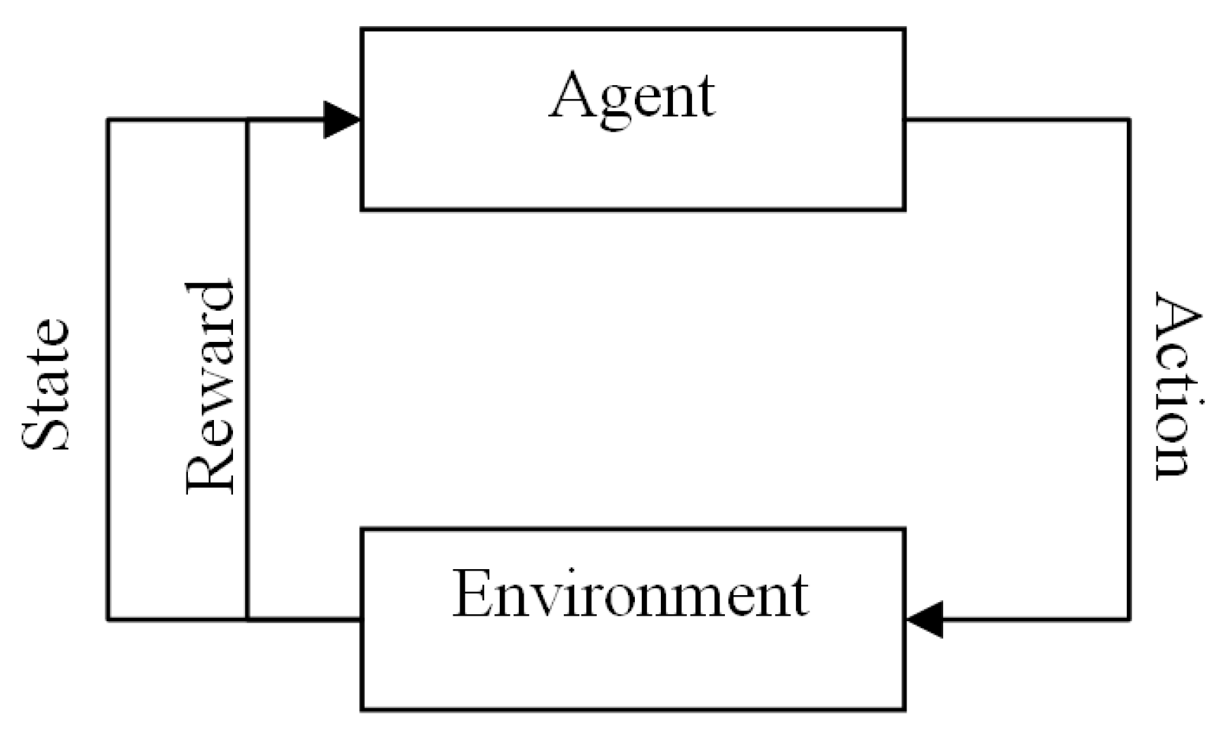
The basic idea of RL can simply be described as a learning agent interacting with its environment to achieve a goal [50]. In reservoir operations, the agent is the operator of a reservoir who makes the decisions over the release (as the action) based on a policy while the state space consists of a set of discrete values of storage.
Beyond the agent and the environment, there are four main sub-elements in RL: a policy, a reward function, a value function, and optionally a model of the environment [50]. The model components of RL determine the next state and the reward of the environment based on a mathematical function. Figure 1 illustrates a schematic perspective of RL.
2.5.1. Action-Taking Policy
The chance of taking an action in a specific state is actually a trade-off between exploration (taking an action randomly) and exploitation (taking the best action), which leads to four common action policies in the literature: random, greedy, ε-greedy and Softmax. In the random policy, there is no action preference. In the ε-greedy policy, greedy action () in each state is chosen most of the time; however, once in a while, the agent tries to choose an action in the set of admissible actions with the probability of where is the probability of taking non-greedy actions and is the set of admissible actions for state . In the greedy policy, the agent picks the best one among all admissible actions in each iteration, with respect to the last estimate of the action-value function for all admissible actions in the respective state. In contrast to the greedy policy, the Softmax policy derived from the Boltzmann’s distribution can be defined in which the proportion of exploration versus exploitation changes as the process of learning continues.
2.5.2. Admissible Actions
The agent should choose an action among candidate actions, which are called possible actions. Evaluation of all state-action pairs is computationally expensive and makes the learning process inefficient. According to the stochastic environment of reservoir operations, some actions might be infeasible to take in some conditions of stochastic variables (e.g., minimum inflow and maximum evaporation) and some are always infeasible. One may define the set of admissible actions based on the worst condition of stochastic variables. However, adopting a such pessimistic approach [42] limits the number of admissible actions, eliminating some actions which might be infeasible in rare conditions; so it is not efficient in terms of finding the optimal policy. Considering the best possible conditions of stochastic variables, the set of admissible actions can be defined using an optimistic approach.
2.5.3. Q-Learning
Q-learning [51] is an RL formulation which has been derived from the formulation of SDP. The value function in SDP is substituted with an action-value function, which is a value defined for every pair of action-states, instead of every state in the value function. Since the learning process is implemented by direct interaction with the environment, value functions have to be updated after each interaction. To find an updated value function based on the Bellman equation, all admissible actions in the respective state and period must be tested with respect to this equation, and the best value is chosen as a new value function. Therefore, we can introduce another terminology called action-value function, , demonstrating the expected accumulated reward when a decision maker starts from state and takes action . Using these new values, the formulation of SDP in the Bellman equation can be written as follows:
where is the immediate reward in period when the action is taken for the transition from state to state , and and are admissible actions and the best one with respect to the next state , respectively.
As demonstrated in Equation (6), the action-value function is the expected value of the sequence of data in the form of . Using the Robbins–Monro algorithm [52], it is simple to find a new formulation as follows:
where is called the learning parameter. Q-learning is a model-free algorithm in which the transition probabilities are not used for updating the action values.
2.6. Aggregation/Decomposition Reinforcement Learning (–-RL)
In this section, a new method, namely aggregation/decomposition RL (AD-RL) is proposed in which Q-learning, is used jointly with AD-DP method. Furthermore, the way of using aggregation/decomposition has been derived from [21] which was generalized in [25].
As mentioned above, Archibald et al. [21] proposed an aggregation/decomposition method in which the original problem should be decomposed to n sub-problems where n is the number of reservoirs. All these sub-problems can be individually solved using SDP or Q-learning. The release of each actual reservoir in each sub-problem is a function of states: the beginning storage of focus (actual) reservoir, the total beginning storage of upstream and non-upstream reservoirs. This means that two virtual reservoirs are assumed to be connected to the actual reservoir in which one is stated in its upstream and the other is in its downstream. As has been explained in Archibald’s technique [21], to decompose the original problem, the upstream and non-upstream should be properly defined. In this decomposition technique, the upstream reservoirs are initially specified. The rest of the reservoirs are, therefore, non-upstream reservoirs. Based on his definition, the upstream reservoirs of an actual reservoir in a sub-problem are those whose releases directly or indirectly reach the focus (actual) reservoir. We defined the non-upstream reservoirs as those which directly or indirectly receive the release from the focus (actual) reservoir. The rest of the reservoirs are upstream ones. Based on some numerical examples, we found that the new definition of virtual reservoirs would end up with a superior release policy in SDP or Q-learning.
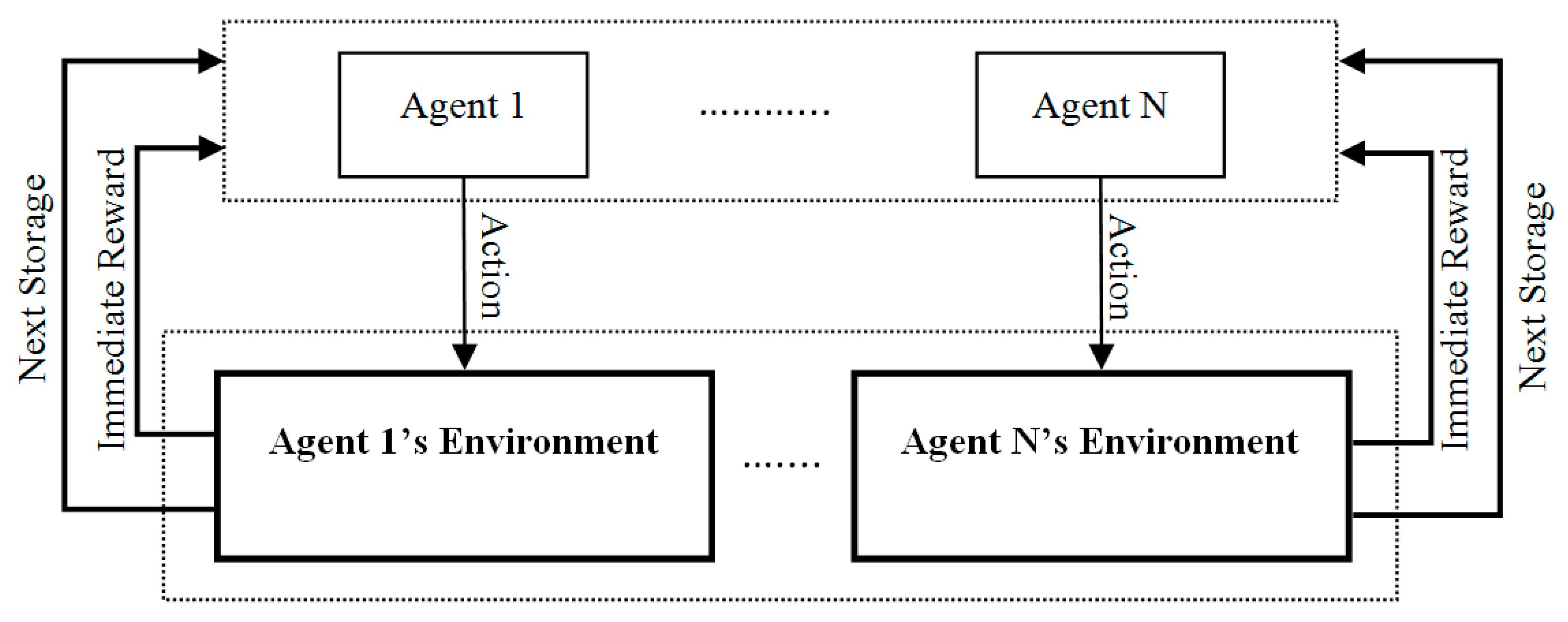
Indeed, there are different interrelated sub-problems in AD-RL that are connected to each other through the releases from actual reservoirs. That means that action (release) taken for each focus (actual) reservoir in a sub-problem in one period is used as an input to the actual reservoir in the next sub-problem in the same period. Therefore, it can be assumed that every sub-problem is conducted by a specific agent and all these agents could share their information through their releases in every interaction of the learning process in AD-RL. Therefore, AD-RL might be interpreted as a multi-agent RL algorithm in which every agent should make a proper decision using its own information and the information received from other agents, including releases and the beginning storages for their respective actual reservoirs. Moreover, the feedback for each agent in the next stage (e.g., the next period) comes from the respective agent and other agents after making their decisions. This feedback includes the next end-of-period storages and the immediate reward for all actual reservoirs in the sub-problems. In other words, each agent should be individually trained until it converges in a steady-state situation in which an optimal policy for that agent can be obtained. The schematic way of training is illustrated in Figure 2.
As illustrated in Figure 2, each agent should interact directly with a specific environment; however, it has indirect interaction with other environments pertinent to other agents. In other words, AD-RL can be projected to a traditional RL in which there are multiple agents (the upper dotted-line box in Figure 2) and multiple environments (the lower dotted-line box in Figure 2) instead of having a single agent and single environment. Therefore, at the time of decision making, each agent should access the beginning storages of all reservoirs. The training part for each agent (updating the action-value functions) should be individually accomplished. The immediate rewards used in the training part for one specific agent come from the reservoir which is related to that agent and from the non-upstream reservoirs that are related to other agents. The developed algorithm (AD-RL) can be summarized as the following steps:
Step 1—The original problem is decomposed to some sub-problems in which the first sub-problem starts for the most upstream reservoir where no releases flow to that reservoir. The last sup-problem is, therefore, one with no downstream reservoirs. As previously mentioned, for each sub-problem, there are two virtual reservoirs: upstream and non-upstream reservoirs. The non-upstream reservoirs should be initially defined. The rest of the reservoirs are upstream reservoirs.
Step 2—For each sub-problem, the states for the respective agent should be defined as follows:
- The beginning storage of focus (actual) reservoir ()
- The summation of beginning storage of all non-upstream reservoirs ()
- The summation of beginning storage of all upstream reservoirs ()
Step 3—all admissible actions (releases), , should be properly defined (based on the optimistic or the pessimistic procedure)
Step 4—Initialize the values of Q-factor for each agent i in all possible state-action pairs
Step 5—Start with initial beginning storages for all reservoirs () and set
Step 6—For all agents,
- Calculate the beginning storages of upstream () and non-upstream () reservoirs.
- Take an action (release) using one of the action-taking policies such as Softmax, ε-greedy, greedy, or random. For instance, if using ε-greedy policy, the probability of release () from reservoir in period in state is calculated as follows:
Step 7—The next state of the actual reservoir in every sub-problem is calculated for all agents using the respective balance equation as the dynamic of the system.
where is the total releases to focus (actual) reservoir from its upstream reservoirs. The decision taken by an agent () in a sub-problem might not be feasible because the storage bounds are not satisfied. In this situation, the next state (the end-of-period storages) are replaced with the respective maximum or the minimum storages, and the releases are revised using the balance equation. Note that the final releases after revision process are used for computing the immediate rewards while the actions (releases before the revision process) are used for training (i.e., updating Q-factors).
Step 8—update the Q-factors for all agents as follows:
where is the reward used to update Q-factors for each action-state pair. There are two types of immediate reward for each agent in every sub-problem: actual and virtual. In the first type, the immediate reward of each agent is considered. Whereas the release from one reservoir might be used multiple times in the downstream, in the virtual type of immediate reward for each agent the benefits of this release should be calculated multiple times in those reservoirs which directly or indirectly receive this flow. For example, where all reservoirs generate power, the release from the most upstream reservoir can contribute the power generation multiple times with different benefit functions in all downstream reservoirs. The total immediate reward for every agent in the respective sub-problem is the summation of actual and virtual immediate rewards.
Step 9—If the stopping criterion is not satisfied, increment t and repeat steps 6–8; otherwise, go to the next step.
Step 10—Find the decision policy using the following equation:
3. Problem Settings and Results
3.1. Case Study: Parambikulam–Aliyar Project (PAP)
We consider the Parambikulam–Aliyar Project (PAP) from India as this multi-reservoir system has been studied using AD-DP and FP methods in [28,49,53], respectively. We provide only the minimum details that are interesting to know here about the system and to correspond with the numbering of reservoirs different here than in [53]; detailed explanations of these reservoirs, their data and corresponding benefits and policies can be obtained from the above works. For the purpose of comparing results with those of four other methods reported in the literature, we use the same problem and objective functions, although that is not a restriction of the AD-RL method. In other words, any other highly non-linear or even discontinuous objective functions can easily be handled by the proposed model as RL is basically a simulation-based technique.
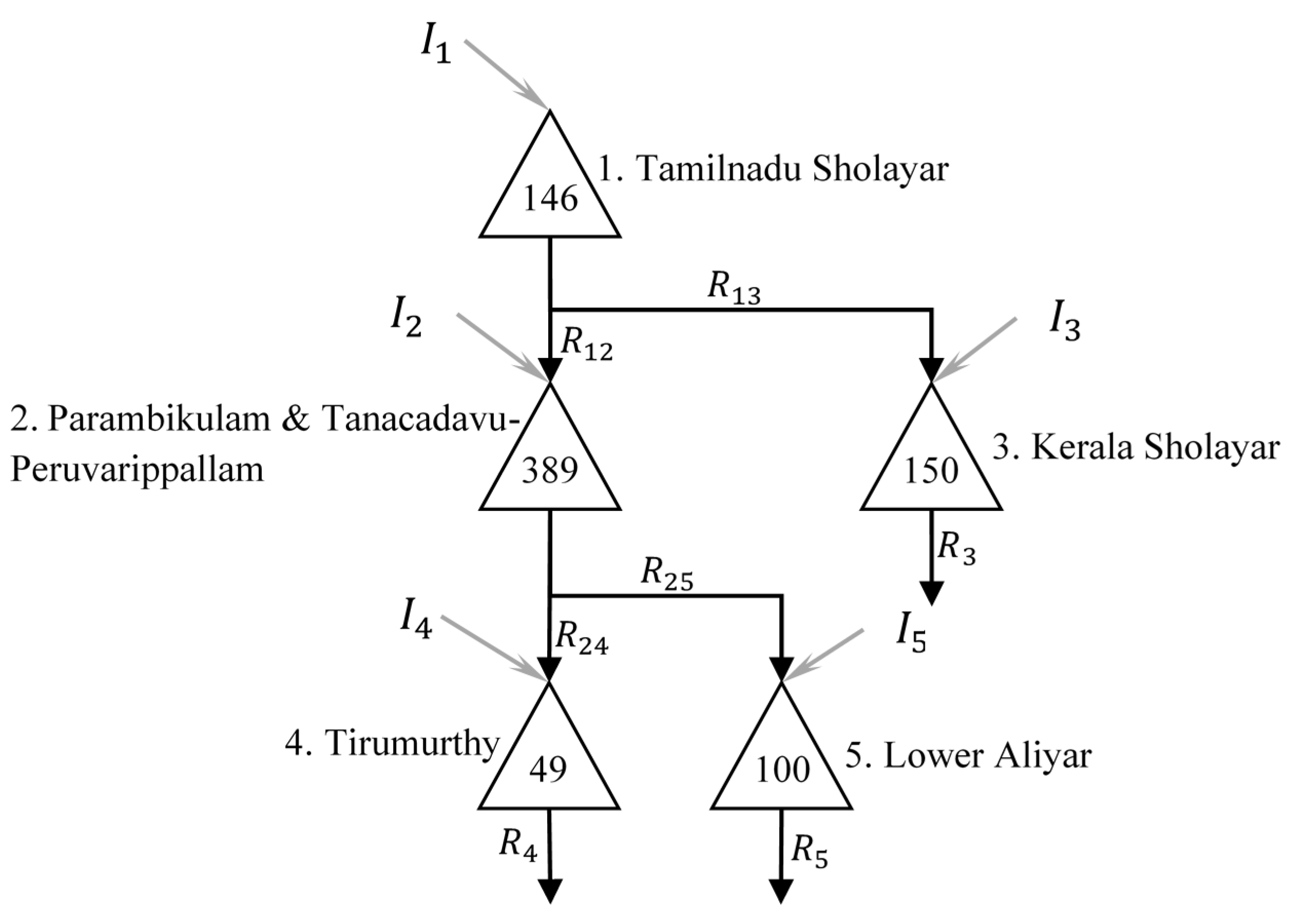
PAP, as studied, is presented in Figure 3. The PAP system comprises of two series of reservoirs in which the left-side reservoirs are more important in terms of the volume of inflow and demands (i.e., the demands and inflows are remarkably high compared to other side). The number inside the triangle depicting each reservoir in Figure 3 represent the live capacities, which can be considered as the maximum storage volume and the minimum (live) storage is zero. The subscript of inflow also represents the index of the reservoir and is used later for explanations.
The main purpose of this project is to conduct water from western slopes of Anamalai Mountains to irrigate the eastern arid area in two states (Tamilnadu and Kerala), and hydropower and fishing benefits are the secondary incomes of the project. Many operating constraints exist agreed upon in the inter-stage agreement between these two different states that should be taken into consideration for constructing any optimization model; the details are not provided here and are available in the original papers. The objective function is defined as;
where is the benefit per unit release which is given in Table 1 and is useful later to understand MAM-DP’s objective function. Note that the above simple linear objective function has been chosen to be exactly the same as the objective function used in the literature for other methods to which we compare our proposed model, and it is not a restriction.
It is worth noting that 20% loss should be considered for all releases flowing from the third reservoir (Paramabikulam reservoir) to the fourth reservoir (Tirumurthy) because of the long tunnel used for water flow between these reservoirs.
The lower release bounds are set to zero for all periods. Table 2 also illustrates the upper bounds for all different connections in the PAP case study (i.e., the release from reservoir to reservoir ). It is assumed that these bounds are the same for 12 months. The diagonal elements in this table indicate the total maximum releases for each of the five reservoirs.
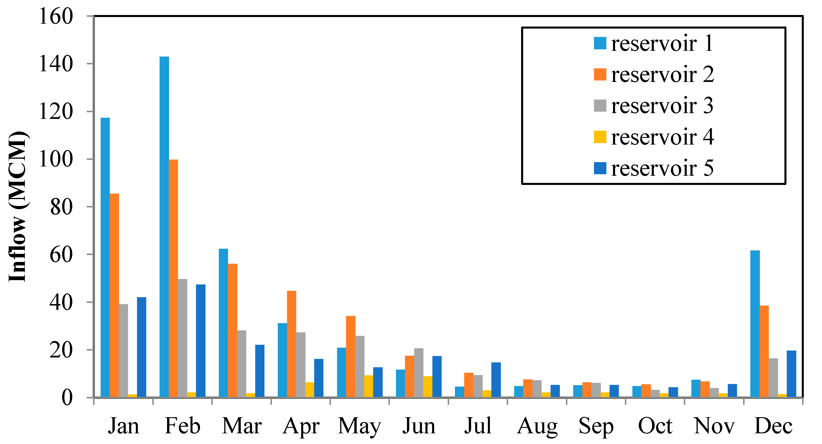
The hydrological data available on a monthly basis for the five reservoirs is in Figure 4. The average monthly inflows to the first, second, third and fifth reservoirs are almost the same in which the rainy season starts from December to May. However, the main proportion of rainfall in the fourth reservoir occurs during the monsoon period (from May to September).
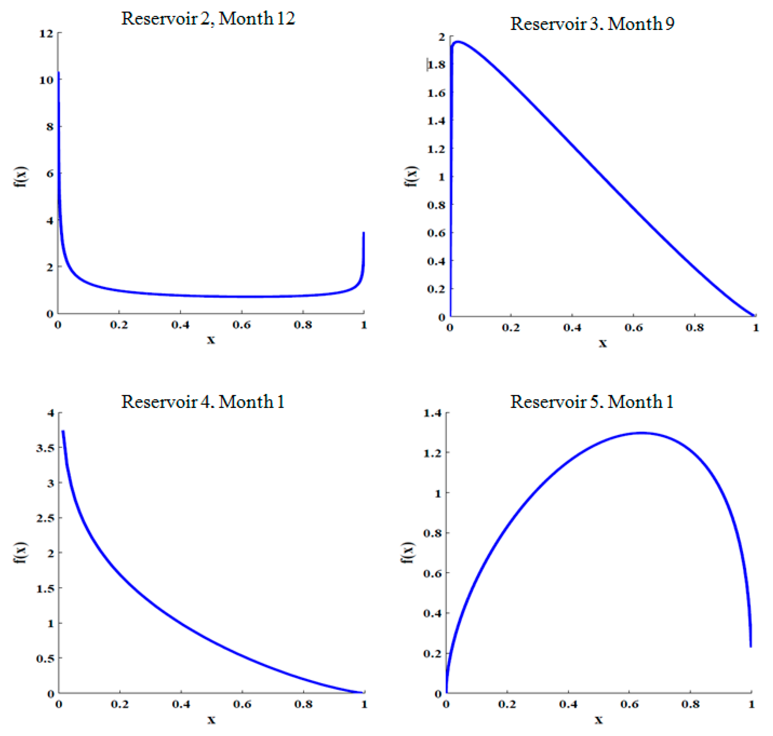
Given the available inflows for each month and the non-normal highly skewed nature of the inflows, the Kumaraswamy distribution was found to be the best fit and a few examples are shown in Figure 5.
Furthermore, based on the nature of PAP case study, there are high correlations between the first reservoir (Tamilnadu Sholayar), the second reservoirs (Parambikalami and Tunacadavu-Peruvarippallam), the third reservoir (Lower Aliyar) and the fifth reservoir (Kerala Sholayar) in terms of natural inflows (Table 3). The inflow to reservoir 4 is independent of other reservoirs’ inflows.
The PAP project is solved using three other different optimization methods, including the MAM-DP, AD-DP and FP techniques in order to verify the performance of the proposed AD-RL. Two different methods of aggregation/decomposition are used in MAM-DP and AD-DP which are explained in the following sub-sections.
3.2. MAM-DP Method Applied to Parambikulam–Aliyar Project (PAP)
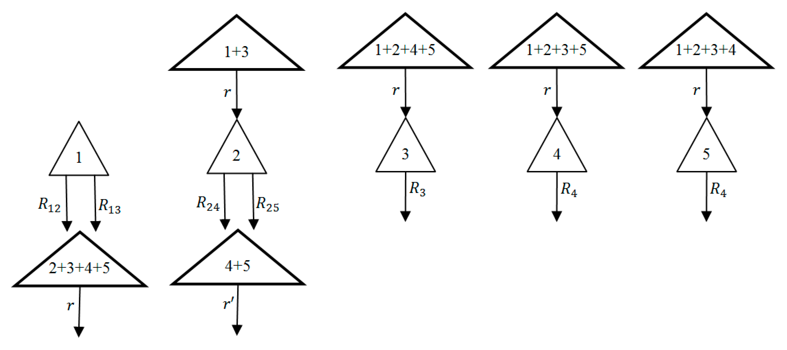
As observed in Figure 6, the PAP problem can be decomposed into four two-reservoir sub-problems for using the 2-level MAM-DP [28]. The values , and are the releases whose conditional probabilities should be calculated from the respective sub-problems. Having solved all sub-problems, the optimal policy for the whole PAP case study can be obtained using the results of all sub-problems’ policies ( and from sub-problem 1; from sub-problem 2; from sub-problem 3; and from sub-problem 4).
Furthermore, defining an objective function for each sub-problem is a challenging issue. Here, it is assumed that the maximum possible benefit for each sup-problem is achieved from the releases in the downstream reservoirs. For instance, in the first period the benefit per unit release for in the first sub-problem is 1.95 (the sum of the benefit per unit release from reservoirs 1, 2 and 4).
3.3. AD-DP Method Applied to PAP Project
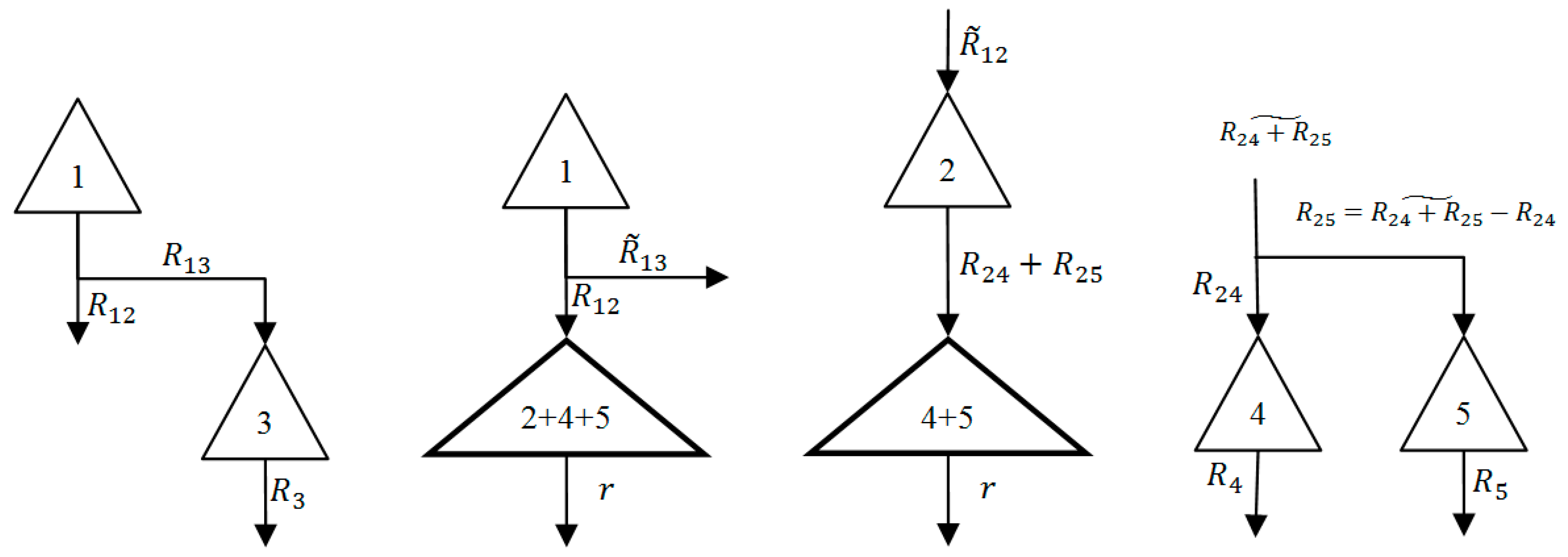
All sub-problems of the PAP project using the AD-DP [21] aggregation method are demonstrated in Figure 7. The reservoir with a thick borderline in each sub-problem is a virtual reservoir whose release is not what actually occurs in reality. For instance, the release out of virtual reservoirs 1 and 3 in the second sub-problem does not really flow into reservoir 2, and it is divided between reservoirs 2 and 3.
As illustrated in Figure 7, the first sub-problem consists of two state variables (the storage of reservoir 1 and the storage of virtual reservoir which is made up from four reservoirs 2, 3, 4 and 5) and three decision variables (the next storage of the virtual reservoir, release from reservoir 1 to reservoir 2 and release from reservoir 1 to reservoir 3). The second sub-problem comprises three state variables and four decision variables. Other sub-problems have two state variables and two decision variables. Furthermore, for these sub-problems, one more assumption (in addition to the one explained in the section on AD-DP regarding the division of storages of the virtual reservoirs) should be taken into consideration in which the release from each virtual reservoir with more than one outlet downstream (e.g., reservoirs 1 and 2) should be proportionally divided based on the respective capacity of the outlets.
3.4. Fletcher–Ponnambalam (FP) Method Applied to PAP
In the FP [17] method, having assumed a linear decision rule, the first and the second moments of storages are available in analytical forms. Substituting these new moments in the objective function produces an analytical expression for the first and second moments of releases, spills, and deficits of each reservoir in each period. All these expressions are dependent on a single parameter for each reservoir in each period. A non-linear optimization is solved directly for the objective function while the statistical moments of storages, releases and probabilities of containments, spills and deficits are also available for all reservoirs. More details can be seen in [53].
3.5. AD-RL Method
To find a near-optimal policy by the Q-learning algorithm, a proper action-taking policy should be chosen. The discount factor (γ) for the learning step is 0.9 while the respective parameters including the learning factor (α) and ε (in ε-greedy policy) or τ (in Softmax policy) should be accurately set.
As previously mentioned, the main advantage of the Softmax policy is to explore more at the beginning of learning while increasing exploitation as learning continues. This behavior is controlled using the values of Q-factors while converging to the steady-state situation, that is, the action with a greater Q-factor should have a higher chance to be chosen in every interaction. However, while applying this policy, it is observed that the values of all Q-factors become almost close to each other as they converge to the steady-state situation. In other words, Softmax might end up with almost identical probabilities for admissible actions. Therefore, this action-taking policy may lead to a poor performance through converging to a far-optimal operating policy, which our numerical experiments accomplished herein confirmed this result too.
Despite the Softmax policy, in ε-greedy policy, the rate of exploration is constant over the learning process that may not guarantee reaching a near-optimal policy. To tackle this issue, the whole learning process can be implemented as episodic starting, with a big ε in the first episode and decrease the rate in the next episode. An episode comprises a predefined number of years that the learning (simulation) should be implemented. The initial state at the beginning of the learning in every episode can be randomly selected. It is worth mentioning that the value of ε in every episode is constant. To implement this way of learning in the PAP case study, we considered two different parameters: ε1 and ε2. The value of ε1 equals one in the first episode, so there will be no difference between all admissible actions in terms of probability of being selected. Parameter ε2 is the rate of exploration in the last episode, then the rate of exploration for other episodes is determined using a linear function of these two parameters.
The learning factor () is also an important parameter that should be precisely specified. There are different methods to set this parameter [54]. It has been specified based on the number of updating for each action-state pair using the following equation:
where is a smaller-than-one predefined parameter. The role of this parameter is to cope with the asynchronous error in the learning process [54].
We use a robust ANN-based approach to tune the above-mentioned parameters. The respective input data for training the corresponding multilayer perceptron ANN is obtained using a combination of different values chosen for parameters ε2 and . To have a space-filling strategy, the values considered for each parameter should be uniformly distributed over its domain (for example takes values of 0.1, 0.3, 0.5, 0.7 and 0.9). Given the sample values chosen for these parameters presented in Table 4, there will be 25 different input data representing all possible combinations for these parameter values. AD-RL will be implemented then for each individual set of these input combinations 10 times. Given the operating policy for each implementation of Q-learning, one can run the respective simulation to obtain the expected value of the benefit. The expected value () and the semi variance () of all 10 expected values of benefit value obtained from the simulations are calculated using the following equations:
where is the number of runs (10 in our experiments), and and are respectively the mean and semi variance values of objective function obtained by ith run.
Recall that Q-learning is a simulation-based technique. Therefore, it could end up with different operating policies at the end of the learning process because of different sequences of synthetic data being generated over the learning phase. Obtaining more robust results for different runs of Q-learning (less variation of expected values at the end of simulation for different Q-learning implementations) is a good sign for the respective fine-tuned parameter values. To take the robustness of the results into account in ANN training task, one can use a function of the performance criterion ( in our experiments) as a desirable output.
To demonstrate how efficient the proposed tuning procedure is, one of the five reservoirs in the PAP case study (Tamilnadu Sholayar reservoir) is selected which can be considered a one-reservoir problem. Similar to what has been undertaken for training data, Q-learning is implemented for the test data set consisting of 100 data in our experiments, and the respective performance criterion is obtained for each test data. The outputs of the networks for these test data can be found using the trained network. The best outputs obtained from Q-learning and the trained networks are compared then to each other. If all or the most of these two different outputs are the same, we conclude that the training phase for tuning the parameters has been performed appropriately.
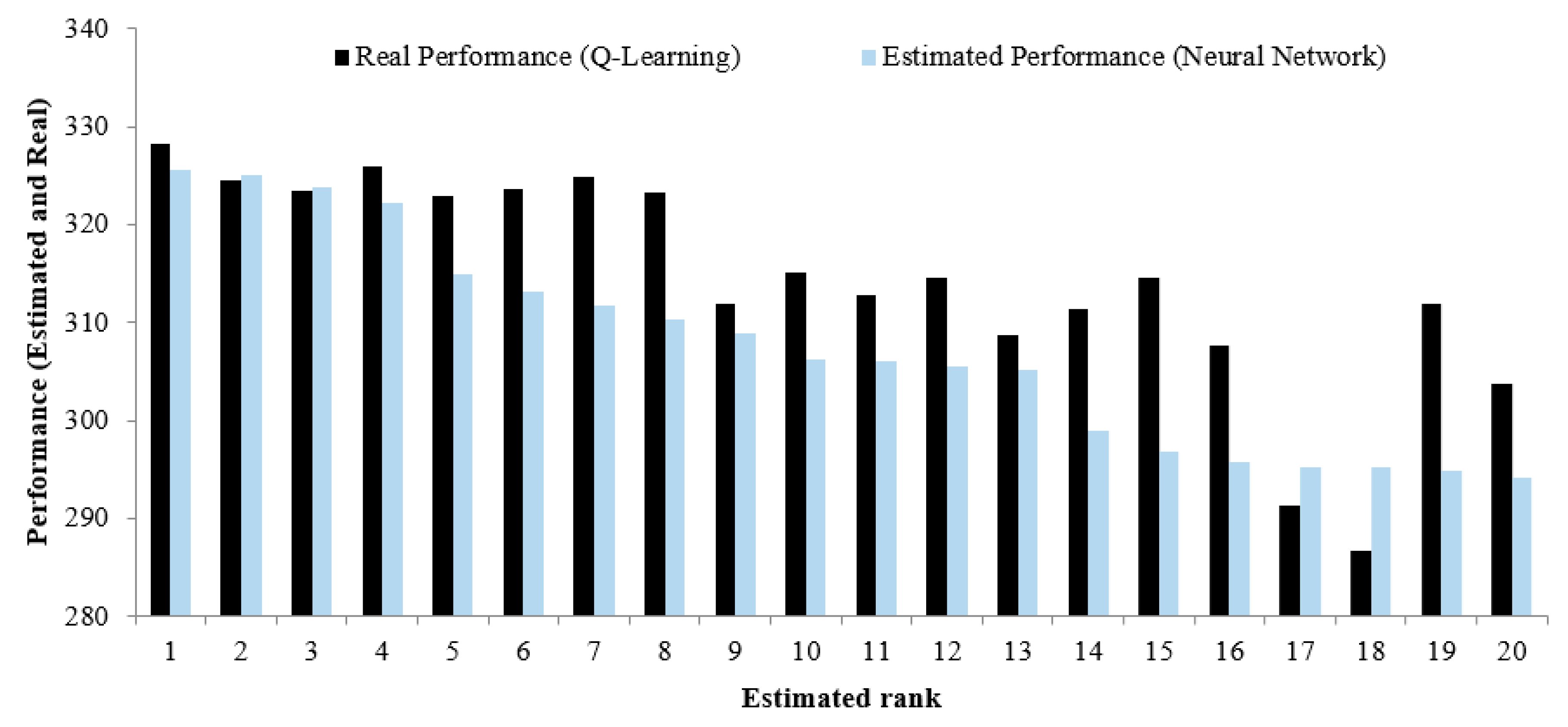
Table 5 demonstrates top- 3, 4, 5, 10, and 15 best sets of parameters in terms of the defined performance criterion (). For instance, 3 out of 5 best sets of parameters based on the output of the trained network are among the 5 best sets of parameters based on the Q-learning approach. Figure 8 illustrates the comparisons between the performance obtained from the neural network for the top 20 sets of parameters and the respective ones based on Q-learning. It shows that the function trained maps the input data to desirable data appropriately. Such a training procedure can, therefore, be used in cases with a larger number of reservoirs.
Having the trained network using 25 examples given in Table 5 for the five-reservoir case study (PAP project), one can select and sort a number of the best parameter sets using 100 test data (Table 6). We used the first set of parameters to implement AD-RL.
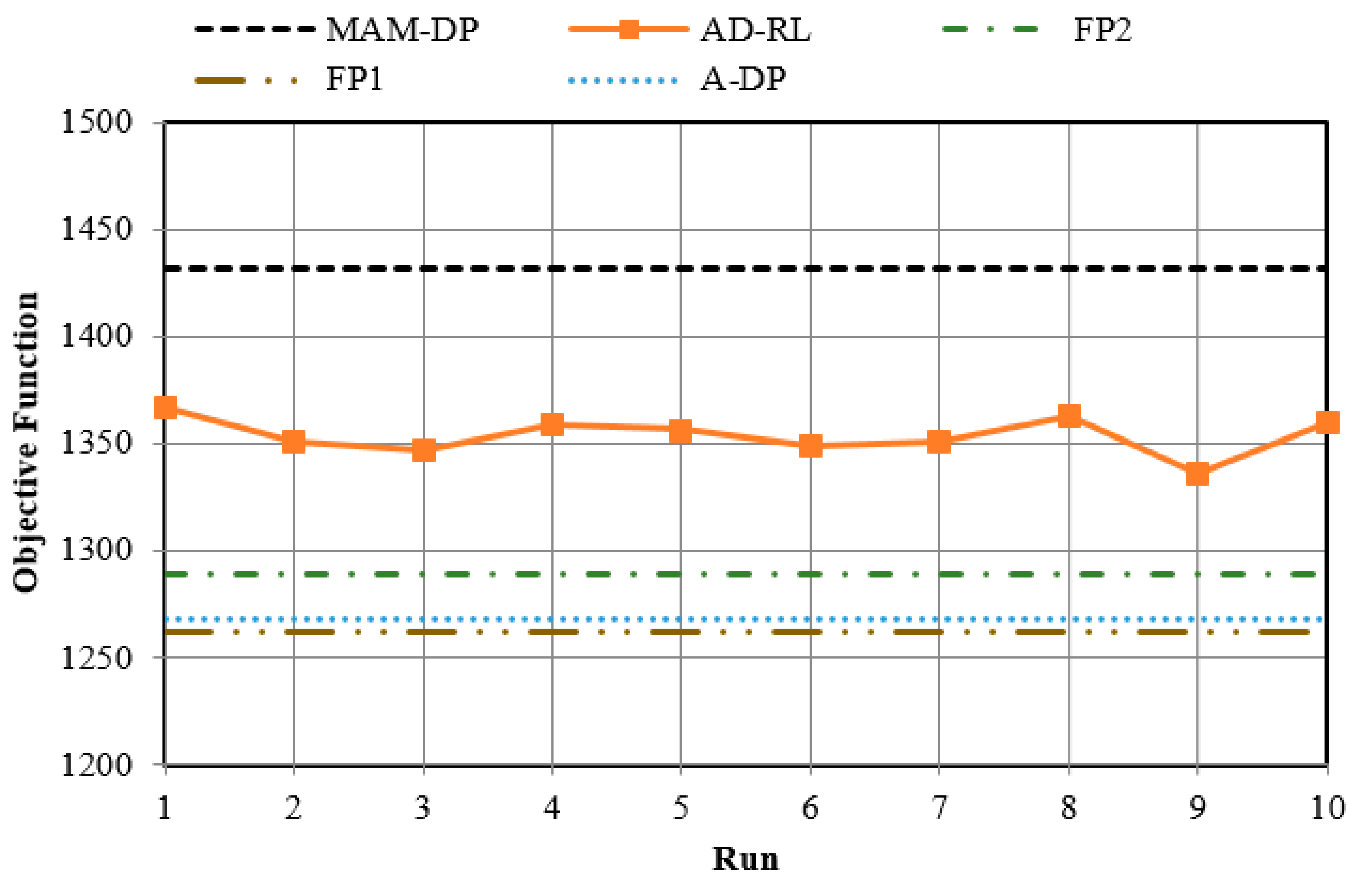
The AD-RL algorithm was implemented 10 times, each with one hundred episodes for the learning process. Each episode comprises 1000 years. Table 7 reports the average and the standard deviation of the annual benefit for all mentioned techniques applied in the PAP case study. It is worth noting that the average and standard deviation reported for the AD-RL method are their mean values obtained from running ten simulations. The AD-DP, MAM-DP, and AD-RL results are also determined by applying them to the same problem (PAP). Finally, the FP1 and FP2 results are from Mahootchi et al. [53] where FP1 and FP2 correspond to different approximations for estimating releases from upstream reservoirs for the Kumaraswamy distributed inflows. See [53] for details.
Figure 9 compares the average benefit for all 10 runs of Q-learning. This is a good verification showing how robust the Q-learning algorithm is. It also verifies that the derived-by-Q learning policy for all different 10 runs outperforms the policies derived by FP and AD-DP.
4. Discussion
In above section, we presented the results of the proposed aggregation decomposition-reinforcement learning (AD-RL) approach for optimizing the PAP multi-reservoir system operations and compared them with those of three other stochastic optimization methods including MAM-DP, FP, and AD-DP. In terms of the average optimality criterion (objective function value), the AD-RL’s solution was the second best result after that of MAM-DP. Because both mean and standard deviations are important, from Table 7 it is clear that the solutions of MAM-DP, AD-RL and FP1 are non-inferior and dominate the solutions of FP2 and AD-DP. Although computational run times are not always the best way to compare complexity in these methods where the number of simulations can be easily changed without much loss in optimality, the AD-RL method was three times faster than MAM-DP for the results presented above. This is important as MAM-DP and AD-RL were the top two ranked methods using mean objective function values. Moreover, as AD-RL was performed using the parameters tuned by a trained ANN, the solutions found by the proposed method in the PAP case study were reasonably robust. In other words, performing the AD-RL technique with different synthetic sequences of data leads to almost similar results. In this regard, assessing the performances of the investigated methods against different reservoir inflow scenarios associated with different runs, the standard deviation of the objective function for the AD-RL method was reasonably good compared to those of other stochastic methods investigated. This risk measure for the AD-RL approach was considerably lower than that resulting from the MAM-DP approach.
Overall, compared to other stochastic optimization methods, the results obtained by the proposed AD-RL approach were promising in terms of the optimality and robustness of the solutions found and the required computational burden.
5. Conclusions
In this paper, an aggregation/decomposition model combined with RL was developed for optimizing multi-reservoir systems operations, in which the whole system is controlled using a number of multiple co-operating agents. This method addresses the so-called dual curses of modeling and dimensionality in SDP. Each agent (operator) finds the best decision (release) for its own reservoir based on its current state and the feedback it receives from other agents represented by two virtual reservoirs, including one each for upstream and non-upstream reservoirs, respectively. An efficient approach based on neural networks was also proposed for tuning the model parameters in order to achieve a robust solution methodology. The developed methodology and original methods that did not use the RL method were applied to the Parambikulam–Aliyar Project (PAP) for which results from other methods were available for comparison.
For the PAP case studied herein, the average performance of the model (based on multiple runs) was compared with the performances of other stochastic optimization techniques, including multilevel approximation dynamic programming (MAM-DP), aggregate dynamic programming (AD-DP), and that of the Fletcher–Ponnambalam (FP) method (reported from the literature). The policies obtained by the AD-RL revealed that the proposed AD-RL approach outperformed FP and AD-DP methods in terms of the objective function criterion while having a comparable performance with MAM-DP but with a less computational time, which can be promising for large-scale problems.
As the proposed method is based on simulation, any other objective functions including non-linear/discontinuous ones can be considered which is a challenging issue for most other stochastic methods and is left for future studies.
Author Contributions
The work presented is mainly based on author M.H.’s MSc. thesis, supervised by authors S.J.M. and M.M. and the following contributions: conceptualization, K.P., M.M. and S.J.M.; methodology, S.J.M. and M.M.; software, M.H., M.M. and K.P.; validation, M.M., S.J.M., M.H. and K.P.; formal analysis, M.H., S.J.M. and M.M.; investigation, M.H., S.J.M. and M.M.; resources, K.P., M.M. and S.J.M.; data curation, K.P. and M.M.; writing—original draft preparation, M.M., S.J.M. and M.H.; writing—review and editing, K.P. and S.J.M.; visualization, M.H.; supervision, S.J.M., M.M. and K.P. All authors have read and agreed to the published version of the manuscript.
Funding
This research received no external funding.
Conflicts of Interest
The authors declare no conflict of interest.
References
- Hiew, K.L.; Labadie, J.W.; Scott, J.F. Optimal operational analysis of the Colorado-Big Thompson project. In Proceedings of the Computerized Decision Support Systems for Water Managers; Labadie, J., Ed.; ASCE: Reston, VA, USA, 1989; pp. 632–646. [Google Scholar]
- Willis, R.; Finney, B.A.; Chu, W.S. Monte Carlo Optimization for Reservoir Operation. Water Resour. Res. 1984, 20, 1177–1182. [Google Scholar] [CrossRef]
- Hiew, K.L. Optimization Algorithms for Large-Scale Multireservoir Hydropower Systems; Colorado State University: Fort Collins, CO, USA, 1987. [Google Scholar]
- Tejada-Guibert, J.A.; Stedinger, J.R.; Staschus, K. Optimization of Value of CVP’s Hydropower Production. J. Water Resour. Plan. Manag. 1990, 116, 52–70. [Google Scholar] [CrossRef]
- Arnold, E.; Tatjewski, P.; Wołochowicz, P. Two Methods for Large-Scale Nonlinear Optimization and Their Comparison on a Case Study of Hydropower Optimization. J. Optim. Theory Appl. 1994, 81, 221–248. [Google Scholar] [CrossRef]
- Lee, J.H.; Labadie, J.W. Stochastic Optimization of Multireservoir Systems via Reinforcement Learning. Water Resour. Res. 2007. [Google Scholar] [CrossRef]
- Aiken, L.S.; West, S.G.; Pitts, S.C. Multiple Linear Regression; Handbook of Psychology; John Wiley & Sons: Hoboken, NJ, USA, 2003. [Google Scholar]
- Hornik, K.; Stinchcombe, M.; White, H. Multilayer Feedforward Networks are Universal Approximators. Neural Netw. 1989, 2, 359–366. [Google Scholar] [CrossRef]
- Wang, L.-X.; Mendel, J.M. Generating Fuzzy Rules by Learning from Examples. IEEE Trans. Syst. Man. Cybern. 1992, 22, 1414–1427. [Google Scholar] [CrossRef] [Green Version]
- Mousavi, S.; Ponnambalam, K.; Karray, F. Reservoir Operation Using a Dynamic Programming Fuzzy Rule–Based Approach. Water Resour. Manag. 2005, 19, 655–672. [Google Scholar] [CrossRef]
- Mousavi, S.J.; Ponnambalam, K.; Karray, F. Inferring Operating Rules for Reservoir Operations Using Fuzzy Regression and ANFIS. Fuzzy Sets Syst. 2007, 158, 1064–1082. [Google Scholar] [CrossRef]
- Loucks, D.P.; Dorfman, P.J. An Evaluation of Some Linear Decision Rules in Chance-Constrained Models for Reservoir Planning and Operation. Water Resour. Res. 1975, 11, 777–782. [Google Scholar] [CrossRef]
- Alizadeh, H.; Mousavi, S.J.; Ponnambalam, K. Copula-Based Chance-Constrained Hydro-Economic Optimization Model for Optimal Design of Reservoir-Irrigation District Systems under Multiple Interdependent Sources of Uncertainty. Water Resour. Res. 2018, 54, 5763–5784. [Google Scholar] [CrossRef]
- Simonovic, S.P.; Marino, M.A. Reliability Programing in Reservoir Management: 1. Single Multipurpose Reservoir. Water Resour. Res. 1980, 16, 844–848. [Google Scholar] [CrossRef]
- Simonovic, S.P.; Marino, M.A. Reliability Programing in Reservoir Management: 2. Risk-Loss Functions. Water Resour. Res. 1981, 17, 822–826. [Google Scholar] [CrossRef]
- Simonovic, S.P.; Marino, M.A. Reliability Programing in Reservoir Management: 3. System of Multipurpose Reservoirs. Water Resour. Res. 1982, 18, 735–743. [Google Scholar] [CrossRef]
- Fletcher, S.; Ponnambalam, K. Constrained State Formulation for the Stochastic Control of Multireservoir Systems. Water Resour. Res. 1998, 34, 257–270. [Google Scholar] [CrossRef]
- Fletcher, S.; Ponnambalam, K. Stochastic Control of Reservoir Systems Using Indicator Functions: New Enhancements. Water Resour. Res. 2008, 44, 44. [Google Scholar] [CrossRef]
- Mahootchi, M. Storage System Management Using Reinforcement Learning Techniques and Nonlinear Models. Ph.D. Thesis, University of Waterloo, Waterloo, ON, Canada, January 2009. [Google Scholar]
- Thomas, H.; Watermeyer, P. Mathematical Models: A Stochastic Sequential Approach; Harvard University Press: Cambridge, MA, USA, 1962. [Google Scholar]
- Archibald, T.; McKinnon, K.; Thomas, L. An Aggregate Stochastic Dynamic Programming Model of Multireservoir Systems. Water Resour. Res. 1997, 33, 333–340. [Google Scholar] [CrossRef] [Green Version]
- Cervellera, C.; Chen, V.C.; Wen, A. Optimization of a Large-Scale Water Reservoir Network by Stochastic Dynamic Programming with Efficient State Space Discretization. Eur. J. Oper. Res. 2006, 171, 1139–1151. [Google Scholar] [CrossRef]
- Foufoula-Georgiou, E. Convex Interpolation for Gradient Dynamic Programming. Water Resour. Res. 1991, 27, 31–36. [Google Scholar] [CrossRef]
- Johnson, S.A.; Stedinger, J.R.; Shoemaker, C.A.; Li, Y.; Tejada-Guibert, J.A. Numerical Solution of Continuous-State Dynamic Programs Using Linear and Spline Interpolation. Oper. Res. 1993, 41, 484–500. [Google Scholar] [CrossRef]
- Karamouz, M.; Mousavi, S.J. Uncertainty Based Operation of Large Scale Reservoir Systems: Dez and Karoon Experience. J. Am. Water Resour. Assoc. 2003, 39, 961–975. [Google Scholar] [CrossRef]
- Mousavi, S.J.; Karamouz, M. Computational Improvement for Dynamic Programming Models by Diagnosing Infeasible Storage Combinations. Adv. Water Resour. 2003, 26, 851–859. [Google Scholar] [CrossRef]
- Philbrick, C.R., Jr.; Kitanidis, P.K. Improved Dynamic Programming Methods for Optimal Control of Lumped-Parameter Stochastic Systems. Oper. Res. 2001, 49, 398–412. [Google Scholar] [CrossRef]
- Ponnambalam, K.; Adams, B.J. Stochastic Optimization of Multi Reservoir Systems Using a Heuristic Algorithm: Case Study from India. Water Resour. Res. 1996, 32, 733–741. [Google Scholar] [CrossRef]
- Saad, M.; Turgeon, A. Application of Principal Component Analysis to Long-Term Reservoir Management. Water Resour. Res. 1988, 24, 907–912. [Google Scholar] [CrossRef]
- Saad, M.; Turgeon, A.; Bigras, P.; Duquette, R. Learning Disaggregation Technique for the Operation of Long-Term Hydroelectric Power Systems. Water Resour. Res. 1994, 30, 3195–3202. [Google Scholar] [CrossRef]
- Saad, M.; Turgeon, A.; Stedinger, J.R. Censored-Data Correlation and Principal Component Dynamic Programming. Water Resour. Res. 1992, 28, 2135–2140. [Google Scholar] [CrossRef]
- Stedinger, J.R.; Faber, B.A.; Lamontagne, J.R. Developments in Stochastic Dynamic Programming for Reservoir Operation Optimization. In Proceedings of the World Environmental and Water Resources Congress, Cincinnati, OH, USA, 19–23 May 2013. [Google Scholar]
- Tejada-Guibert, J.A.; Johnson, S.A.; Stedinger, J.R. The Value of Hydrologic Information in Stochastic Dynamic Programming Models of a Multireservoir System. Water Resour. Res. 1995, 31, 2571–2579. [Google Scholar] [CrossRef]
- Turgeon, A. Optimal Operation of Multireservoir Power Systems with Stochastic Inflows. Water Resour. Res. 1980, 16, 275–283. [Google Scholar] [CrossRef]
- Turgeon, A. A Decomposition Method for the Long-Term Scheduling of Reservoirs in Series. Water Resour. Res. 1981, 17, 1565–1570. [Google Scholar] [CrossRef]
- Pereira, M.V.F. Optimal Stochastic Operations Scheduling of Large Hydroelectric Systems. Int. J. Electr. Power Energy Syst. 1989, 11, 161–169. [Google Scholar] [CrossRef]
- Pereira, M.V.F.; Pinto, L.M.V.G. Multi-Stage Stochastic Optimization Applied to Energy Planning. Math. Program. 1991, 52, 359–375. [Google Scholar] [CrossRef]
- Poorsepahy-Samian, H.; Espanmanesh, V.; Zahraie, B. Management. Improved Inflow Modeling in Stochastic Dual Dynamic Programming. J. Water Resour. Plan. Manag. 2016, 142, 04016065. [Google Scholar] [CrossRef]
- Rougé, C.; Tilmant, A. Using Stochastic Dual Dynamic Programming in Problems with Multiple Near-Optimal Solutions. Water Resour. Res. 2016, 52, 4151–4163. [Google Scholar] [CrossRef] [Green Version]
- Zhang, J.L.; Ponnambalam, K. Stochastic Control for Risk Under Deregulated Electricity Market—A Case Study Using a New Formulation. Can. J. Civ. Eng. 2005, 32, 719–725. [Google Scholar] [CrossRef]
- Kelman, J.; Stedinger, J.R.; Cooper, L.A.; Hsu, E.; Yuan, S.Q. Sampling Stochastic Dynamic Programming Applied to Reservoir Operation. Water Resour. Res. 1990, 26, 447–454. [Google Scholar] [CrossRef]
- Mahootchi, M.; Tizhoosh, H.; Ponnambalam, K. Opposition-based reinforcement learning in the management of water resources. In Proceedings of the IEEE International Symposium on Approximate Dynamic Programming and Reinforcement Learning, Honolulu, HI, USA, 1–5 April 2007; pp. 217–224. [Google Scholar]
- Castelletti, A.; Pianosi, F.; Restelli, M. A Multiobjective Reinforcement Learning Approach to Water Resources Systems Operation: Pareto Frontier Approximation in a Single Run. Water Resour. Res. 2013, 49, 3476–3486. [Google Scholar] [CrossRef] [Green Version]
- Bhattacharya, B.; Lobbrecht, A.; Solomatine, D. Neural Networks and Reinforcement Learning in Control of Water System. J. Water Resour. Plan. Manag. 2003, 129, 458–465. [Google Scholar] [CrossRef]
- Castelletti, A.; Galelli, S.; Restelli, M.; Soncini-Sessa, R. Tree-Based Reinforcement Learning for Optimal Water Reservoir Operation. Water Resour. Res. 2010, 46, W09507. [Google Scholar] [CrossRef]
- Pianosi, F.; Castelletti, A.; Restelli, M. Tree-Based Fitted Q-Iteration for Multi-Objective Markov Decision Processes in Water Resource Management. J. Hudroinform. 2013, 15, 258–270. [Google Scholar] [CrossRef] [Green Version]
- Bertoni, F.; Giuliani, M.; Castelletti, A. Integrated Design of Dam Size and Operations via Reinforcement Learning. J. Water Resour. Plan. Manag. 2020, 146, 04020010. [Google Scholar] [CrossRef]
- Bellman, R. Dynamic Programming and Lagrange Multipliers. Proc. Natl. Acad. Sci. USA 1956, 42, 767. [Google Scholar] [CrossRef] [PubMed] [Green Version]
- Ponnambalam, K.; Adams, B.J. Experiences with integrated irrigation system optimization analysis. In Proceedings of the Irrigation and Water Allocation (Proc., Vancouver Symposium); IAHS: Wallingford, UK, 1987; pp. 229–245. [Google Scholar]
- Sutton, R.S.; Barto, A.G. Reinforcement Learning: An Introduction; MIT Press: Cambridge, MA, USA, 1998; Volume 1. [Google Scholar]
- Watkins, C.J.C.H.; Dayan, P. Q-Learning. Mach. Learn. 1992, 8, 279–292. [Google Scholar] [CrossRef]
- Robbins, H.; Monro, S. A Stochastic Approximation Method. Ann. Math. Stat. 1951, 22, 400–407. [Google Scholar] [CrossRef]
- Mahootchi, M.; Ponnambalam, K.; Tizhoosh, H. Operations Optimization of Multireservoir Systems Using Storage Moments Equations. Adv. Water Resour. 2010, 33, 1150–1163. [Google Scholar] [CrossRef]
- Gosavi, A. Simulation-Based Optimization: Parametric Optimization Techniques and Reinforcement Learning; Springer: Berlin/Heidelberg, Germany, 2014; Volume 55. [Google Scholar]
Figure 1.
The schematic view of reinforcement learning.

Figure 2.
Schematic of aggregation/decomposition reinforcement learning (AD-RL) algorithm.

Figure 3.
Parambikulam–Aliyar Project (PAP) system as studied.

Figure 4.
The average monthly inflows in million cubic meter (MCM).

Figure 5.
Examples for the probability density functions of inflows to reservoirs [19].
Figure 5.
Examples for the probability density functions of inflows to reservoirs [19].

Figure 6.
The sub-problems of PAP using the multilevel approximation-dynamic programming (MAM-DP) method [28].
Figure 6.
The sub-problems of PAP using the multilevel approximation-dynamic programming (MAM-DP) method [28].

Figure 7.
The sub-problems of PAP using the aggregation–decomposition dynamic programming (AD-DP) method [28].
Figure 7.
The sub-problems of PAP using the aggregation–decomposition dynamic programming (AD-DP) method [28].

Figure 8.
The estimated and real performance of top 20 sets based on estimated performance.

Figure 9.
The average expected value of the objective function for 10 different runs.


Table 1.
The benefit per unit release.
| Reservoir | Periods | |||||||||||
|---|---|---|---|---|---|---|---|---|---|---|---|---|
| 1 | 2 | 3 | 4 | 5 | 6 | 7 | 8 | 9 | 10 | 11 | 12 | |
| 1 | 0.6 | 1 | 1 | 0.05 | 0.2 | 0.2 | 0 | 0 | 0 | 0 | 0 | 0 |
| 2 | 0.8 | 0.9 | 1 | 0.4 | 0.4 | 0.7 | 0.8 | 0.8 | 0.8 | 0 | 0 | 0 |
| 3 | 0.1 | 0.25 | 0.3 | 0.22 | 0.25 | 0.4 | 0.5 | 0.4 | 0.4 | 0.3 | 0.2 | 0.2 |
| 4 | 0.55 | 0.9 | 1 | 0.22 | 0.28 | 0.42 | 0.58 | 0.62 | 0.44 | 0 | 0 | 0 |
| 5 | 0.25 | 0.35 | 0.35 | 0.25 | 0.35 | 0.3 | 0.3 | 0.3 | 0 | 0 | 0.2 | 0.25 |
Table 2.
The upper bounds of release.
| Res. 1 | Res. 2 | Res. 3 | Res. 4 | Res. 5 | |
|---|---|---|---|---|---|
| Res. 1 | 173.62 | 123.9 | 49.72 | - | - |
| Res. 2 | - | 115.4 | - | 57.7 | 57.7 |
| Res. 3 | - | - | 66.67 | - | - |
| Res. 4 | - | - | - | 105.12 | - |
| Res. 5 | - | - | - | - | 49.23 |
Table 3.
The cross-correlation between inflows to reservoirs.
| Res. 1 | Res. 2 | Res. 3 | Res. 4 | Res. 5 | |
|---|---|---|---|---|---|
| Res. 1 | 1.0 | 0.8 | 0.8 | −0.1 | 0.9 |
| Res. 2 | 0.8 | 1.0 | 0.8 | 0.1 | 0.8 |
| Res. 3 | 0.8 | 0.8 | 1.0 | 0.3 | 0.7 |
| Res. 4 | −0.1 | 0.1 | 0.3 | 1.0 | 0.0 |
| Res. 5 | 0.9 | 0.8 | 0.7 | 0.0 | 1.0 |
Table 4.
Values of , , for making input data.
| Parameters | Values | ||||
|---|---|---|---|---|---|
| B | 0.1 | 0.3 | 0.5 | 0.7 | 0.9 |
| Initial exploration factor | 1 | 1 | 1 | 1 | 1 |
| Final exploration factor | 0 | 0.1 | 0.3 | 0.5 | 0.7 |
Table 5.
The number of the same sets of parameters according to estimated-by-artificial neural network (ANN) and actual (obtained-by-Q learning) performances for top- set.
Table 5.
The number of the same sets of parameters according to estimated-by-artificial neural network (ANN) and actual (obtained-by-Q learning) performances for top- set.
| 3 | 4 | 5 | 10 | 15 | |
| The number of the same sets in top n sets | 1 | 3 | 3 | 9 | 14 |
Table 6.
Top three parameter sets obtained by the ANN-based parameter tuning approach for AD-RL algorithm applied to PAP.
Table 6.
Top three parameter sets obtained by the ANN-based parameter tuning approach for AD-RL algorithm applied to PAP.
| Rank | Performance Criteria | ε2 | B. |
|---|---|---|---|
| 1 | 1347.447 | 0.3 | 0.9 |
| 2 | 1346.325 | 0.4 | 0.9 |
| 3 | 1345.93 | 0.2 | 0.9 |
Table 7.
The average expected value and the standard deviation of annual benefit.
| Methods | Ave. | Std. |
|---|---|---|
| MAM-DP * | 1432.2 | 249.6 |
| AD-RL * | 1353.9 | 224.1 |
| FP2 | 1289.5 | 230.4 |
| FP1 | 1262.5 | 211 |
| AD-DP * | 1268.0 | 231.6 |
* Results from the methods implemented in this paper.
© 2020 by the authors. Licensee MDPI, Basel, Switzerland. This article is an open access article distributed under the terms and conditions of the Creative Commons Attribution (CC BY) license (http://creativecommons.org/licenses/by/4.0/).
Share and Cite
MDPI and ACS Style
Hooshyar, M.; Mousavi, S.J.; Mahootchi, M.; Ponnambalam, K. Aggregation–Decomposition-Based Multi-Agent Reinforcement Learning for Multi-Reservoir Operations Optimization. Water 2020, 12, 2688. https://doi.org/10.3390/w12102688
AMA Style
Hooshyar M, Mousavi SJ, Mahootchi M, Ponnambalam K. Aggregation–Decomposition-Based Multi-Agent Reinforcement Learning for Multi-Reservoir Operations Optimization. Water. 2020; 12(10):2688. https://doi.org/10.3390/w12102688
Chicago/Turabian StyleHooshyar, Milad, S. Jamshid Mousavi, Masoud Mahootchi, and Kumaraswamy Ponnambalam. 2020. "Aggregation–Decomposition-Based Multi-Agent Reinforcement Learning for Multi-Reservoir Operations Optimization" Water 12, no. 10: 2688. https://doi.org/10.3390/w12102688
Note that from the first issue of 2016, this journal uses article numbers instead of page numbers. See further details here.