Technical Efficiency of China’s Agriculture and Output Elasticity of Factors Based on Water Resources Utilization
by
 , and
, and
Shiliang Yang
1,2,3,* ,
,
Huimin Wang
1,2,*,
Jinping Tong
1,4,
Jianfeng Ma
4,
Fan Zhang
1,2 and
Shijuan Wu
3,5 1
State Key Laboratory of Hydrology Water Resource and Hydraulic Engineering, Hohai University, Nanjing 210098, China
2
Institute of Management Science, Hohai University, Nanjing 210098, China
3
Odette School of Business, University of Windsor, Windsor, ON N9B 3P4, Canada
4
School of Business, Changzhou University, Changzhou 213164, China
5
School of Economics and Management, Fuzhou University, Fuzhou 350108, China
*
Authors to whom correspondence should be addressed.
Water 2020, 12(10), 2691; https://doi.org/10.3390/w12102691
Submission received: 21 August 2020
/
Revised: 21 September 2020
/
Accepted: 23 September 2020
/
Published: 26 September 2020
(This article belongs to the Special Issue The Water-Energy-Food Nexus: Sustainable Development)
Abstract
:A stochastic frontier approach (SFA) model of translog production function was constructed to analyze the growth effect of agricultural production factors on grain production in China. Under the condition of unchanged cultivated land, the agricultural labor, capital, and water were regarded as input elements of the agricultural production function. The maximum likelihood estimation (MLE) method was used to analyze the technical efficiency, output elasticity, substitution elasticity, and relative variability of grain production in China from 2004 to 2018. The results showed that: (1) For the technical efficiency and output elasticity of the input factors of grain production, there were significant differences in different provinces. For example, the water resource was insufficient in Beijing and Shanghai, but the output elasticity of water was high. Heilongjiang was rich in water and had high technical efficiency. For Xinjiang, water was sufficient, but its output elasticity was deficient and the technical efficiency didn’t increase. (2) The overall technical efficiency level was relatively low and was still declining year by year; the output elasticity of water was much greater than that of capital. There was still great potential for grain growth. (3) Optimizing resource allocation and controlling the appropriate ratio of input factors to develop grain production could achieve the maximum benefits. Finally, according to the empirical results, this paper put forward some practical policy suggestions for optimizing the allocation of input factors, especially water and capital, which can ultimately improve agricultural productivity by improving technical efficiency.
1. Introduction
With the accelerated development of agricultural production, capital, labor, water, and land are becoming increasingly scarce [1], fertilizer and pesticide inputs are increasing, and the ecological environment is deteriorating [2]. As part and parcel of corporate social responsibility, water pollution control in grain production also complies with the rise of today’s consciousness of environmental evolutions such as climate change [3,4,5]. Real options are needed to approach to the challenge of grain production sustainability for water resource protection [6]. Realizing the rational allocation of agricultural production factors and protecting water resources is an issue that needs to be solved for the current sustainable growth of grain [7,8]. At the present stage, the growth mode of grain yield in China is excessively dependent on the increase of the input factors [9]. This “extensive” production mode will undoubtedly lead to scale inefficiency, redundant inputs, and waste of resources [10]. Meanwhile, the high-quality labor, capital, water, and other resources required for agricultural production are attracted to urban areas with increasing returns [11]. As a result, it is challenging to achieve coordinated matching of the inputs of agricultural production factors. Therefore, in-depth analysis of the technical efficiency of grain production, the output elasticity, substitution elasticity and variation degree of production factors, and handling of the input–output relationship of agricultural production factors are the key to improving the allocation efficiency of grain production factors in China.
Many research studies have been carried out on this topic. On the one hand, a well-known phenomenon of grain production is that it takes into account the different input factors, such as labor [12], land [13], fertilizer [14,15], machinery [16], multiple crop index [17], plastic sheeting [18], market [19], climate change [20], policy [21,22], and so on, as well as the comparison of the disparity in efficiency and elasticity. For example, Truc Linh [23] considered that productivity growth was strongly correlated with environmental performance. Jose [24] believed that climate conditions, soil irrigation, and other factors affected the agricultural production efficiency of Brazil. At the same time, Shiferawt Holden [25] held that the continuous degradation of soil conditions was an important factor. Vollrath [26] thought that the inequality of cultivated land resource allocation had an impact on agricultural production efficiency. Water pollution in Egypt adversely affected crop yields and agricultural production, reducing technical efficiency [27]. Moreover, the agricultural technical efficiency of Nigeria was 81%, and crop diversity could increase technical efficiency [28]. The region with the highest average technical efficiency was the central region (90%) in India, where the agricultural experience and age were major factors in technical inefficiency [29]. The sum of output elasticity of each production element in the United States was 1.2, which showed the state of increasing returns to scale [30]; the output elasticity of agricultural labor was around 0.5, while the output elasticity of agricultural land was lower than that of labor by as much as 0.2 in Japan [31]; and the difference of output elasticity of agricultural production factors in 127 countries was small, around 0.2 [32].
Different methods and techniques of measurement were used, mainly including data envelopment analysis (DEA) [33,34], stochastic frontier approach (SFA) [35,36], and combining DEA and SFA with other methods. For example, Min et al. [37] calculated that there was a hidden danger of decline in the technical efficiency of Hubei province based on sequence DEA. Mareth et al. [38] used DEA and quantile regression to calculate the technical efficiency score of agricultural growth, while Liu et al. [39] used a three-stage DEA model to compare the production efficiency of Yangxian county and surrounding counties. Victor et al. [40] used SFA, DEA, and generalized cross-entropy (GCE) methods to obtain the importance of resource productivity and subsidies to agricultural technology efficiency. Feng et al. [41] combined the Tobit model to analyze the main influencing factors of grain counties in Jilin Province. Liu [42] used DEA and a nonparametric Malmquist index to analyze and evaluate grain production efficiency in underdeveloped areas of China. Mwangi [43] used the Cobb–Douglas production function to measure the technical efficiency of tomato production and Fan et al. [44] used the translog stochastic frontier production function to measure the frequency distribution of technical efficiency of grain production and the elasticity coefficient of input–output.
However, this appears as a more straightforward problem compared to the input of water, which is even more challenging because grain production is mainly dependent on water resources. In the process of grain production, similar studies were done on water efficiency [45], allocation of grain production factors [46], and the ways to improve production efficiency [47]. We found that grain production efficiency in China was generally low, and the eastern coastal areas generally showed a trend of efficiency reduction [48]. For the estimation of output elasticity of agricultural production factors, labor and capital were the main factors that determined agricultural output [49]. The scarcity of irrigation water would limit grain production, and at the same time, it would induce agricultural technology retrogression and reduce the elasticity of the food supply [50]. Regarding the elasticity of substitution, the development of an agricultural machinery service had a substitution relationship with labor output elasticity and had a complementary relationship with the output elasticity of chemical fertilizers and machinery [51]. The food industry of our country was in a stage of increasing returns to scale with technological progress [52]. Previously published studies have been limited to the qualitative analysis of the input factors of water, and few studies have focused on technical efficiency and output elasticity of the water. It is impossible to plan quantitative quota according to local conditions to realize the optimal allocation of water resources.
To our knowledge, the SFA method could be used as a reference for sample fitting degree and statistical properties through statistical tests compared with the sensitivity of the commonly used DEA method to abnormal data under the condition of large samples [53,54]. Therefore, we propose this method combining the translog production function to estimate the stochastic production frontier and technical efficiency loss function at the same time. Water is one of the most critical inputs for grain growth and agriculture development. It is of interest to know whether the intake of water increased understanding of grain production. This paper aimed to assess the extent to which these factors affect the technical efficiency loss under the premise of being unbiased and effective. It could also effectively estimate the output elasticity, substitution elasticity, and relative variability of grain production. The research can provide a theoretical framework and technical support for comprehensive management, which is of great significance to the development of China’s agriculture. The paper is organized as follows: Section 2 introduces the study area, framework, methodology, and data sources. Section 3 describes the results. The main discussion is presented in Section 4. Section 5 gives the conclusions of the study.
2. Materials and Methods
2.1. Study Area
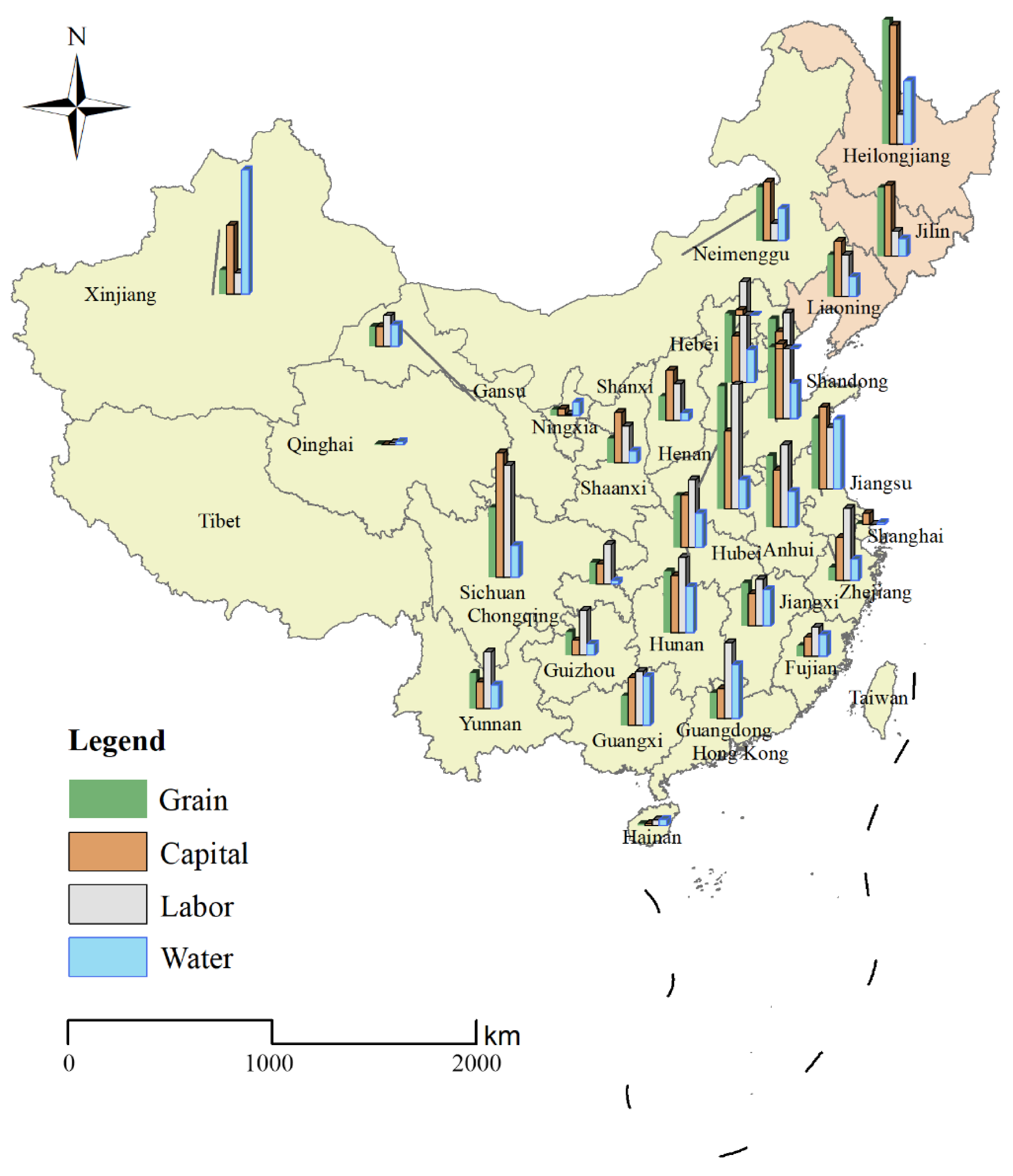
China is a country with a large population and agricultural production. There is a total of 31 provinces in China (Figure 1). The resource endowments and regional structure of grain production in each province are different, and the food output varies greatly. Among them, the Northeast is the main grain production area, including Heilongjiang, Jilin, and Liaoning, and is also one of the world’s three largest black soil regions, accounting for about 20% of the country’s total food output. The abundance or shortage of food in the Northeast is directly related to national food security. It affects the healthy development of China’s economy and social stability. Therefore, the grain production situation of the Northeast is listed separately and compared with the nation.
In the past 18 years, the average annual accumulated grain output of the nation was tons, and that of the Northeast was tons. Among them, the total national yield of soybeans was tons and the Northeast was tons, which accounted for 45.88%. Nearly half of China’s soybeans were produced in the Northeast.
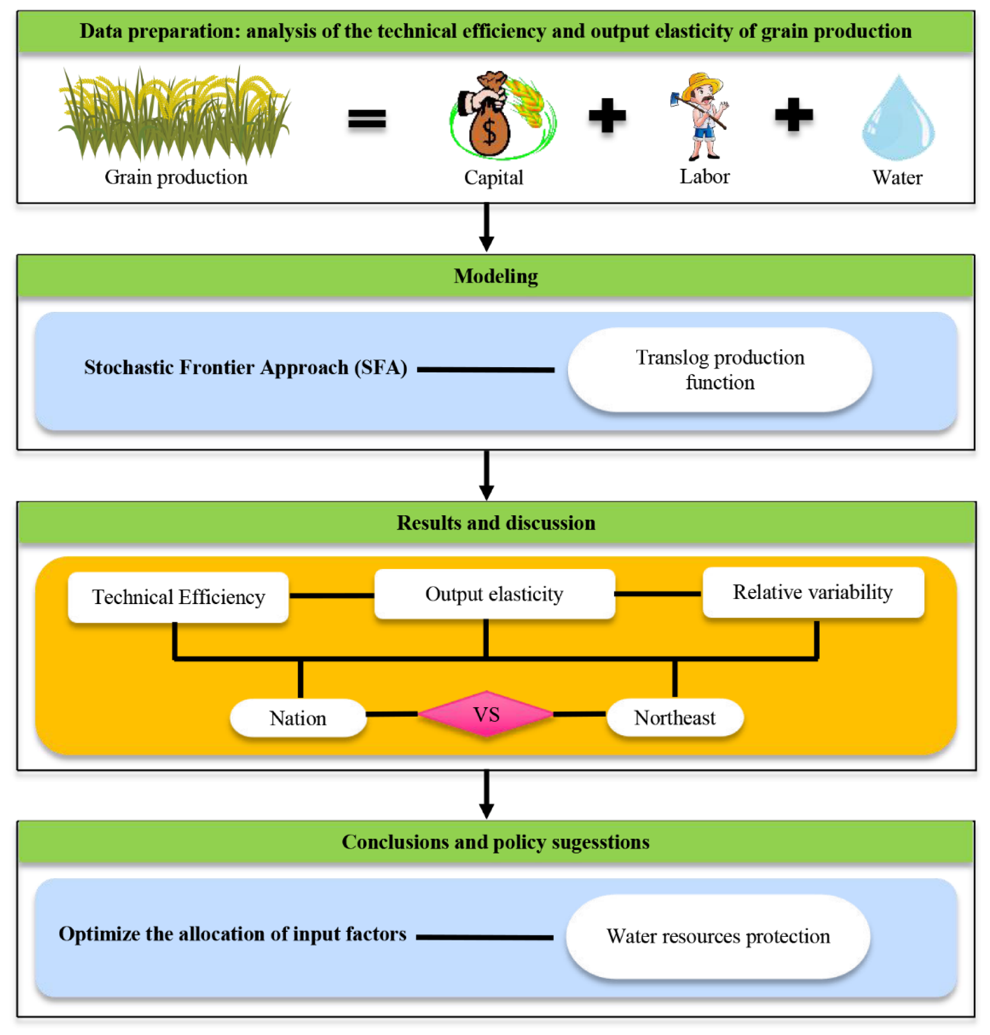
2.2. Operational Framework
To study the growth effect of agricultural production factors on grain production in China, the input factors of agricultural labor, capital, and water resources were considered as the input elements under the condition of unchanged cultivated land conditions. The stochastic frontier approach (SFA) of the translog was constructed to analyze the technical efficiency, output elasticity, substitution elasticity, and relative variability, and compared the situation between the nation and the Northeast to study regional characteristics, and finally, give the corresponding resource optimization allocation, water resources protection policy, and so on. An operational framework is shown (Figure 2).
2.3. Modeling
2.3.1. SFA Model
The method of maximum likelihood estimation (MLE) was used by the SFA model [55] to determine the frontier boundary, which is a random boundary model with a compound disturbance term. Its frontier was random, and the conclusions obtained were closer to the actual situation.
Under the panel data, it is assumed that there are decision making units (DMU) and observation values in the period of time , and each DMU has input and output . The input of the th DMU in period is , the output is , and the production function is , where is the parameter value. According to the stochastic frontier model method, its SFA model can be expressed as:
where, is the error term (also known as random disturbance term), which is composed of two parts: one is , namely the impact of external environmental factors and other random variables on output (also known as random error term); the other is , namely the impact of technical inefficiency on output (also known as the non-negative error term).
Taking the logarithm of both sides of Equation (1), the following linear form can be obtained:
where and obey independent and uncorrelated distribution, in which is the classical noise term obeying the standard normal distribution, while is mostly used as a semi-normal distribution or truncated normal distribution in the calculation of efficiency. The complex disturbance term does not satisfy the classical assumption of least squares estimation, so the ordinary least square (OLS) method can not be used for estimation, and the maximum likelihood estimate (MLE) is adopted.
The model has the following assumptions:
- (1)
- Random error term:
It is mainly caused by uncontrollable factors, such as natural disasters and weather factors.
- (2)
- Non-negative error term:
The truncated normal distribution (the part less than zero is truncated) is taken, and and are independent of each other.
- (3)
- , , and explanatory variable are independent of each other.
2.3.2. Technical Efficiency
Technical efficiency [56] has been improved on the basis of previous research and introduced the concept of time so that the SFA model can evaluate the efficiency of panel data [57]. The representative definition of technical efficiency is given by [58] from the perspective of input in the paper “Measurement of Production Efficiency”. Technical efficiency refers to the percentage of the minimum cost to the actual cost of producing a certain amount of products according to the given input proportion of factors under the condition of constant output scale and market price.
Assuming that the actual output level is and the output at the stochastic frontier is , then the distance between the two is the efficiency loss, also known as the technical efficiency, which is represented by as follows:
where is a parameter used to measure the changes of technical efficiency over time. If is statistically significant, it means that technical efficiency will change significantly over time. indicate that the absolute value of technical efficiency loss becomes smaller, larger, or remains unchanged with time. represents the trend of advanced technological progress. As shown above, and are the mean and standard deviation of technical efficiency loss respectively, namely .
In addition, through the variance of and , there is , is between 0 and 1, which reflects the proportion of technical inefficiency in the random disturbance. If , it means that the output level of the frontier in the model is completely caused by the random disturbance term. That is to say, we do not need to adopt the stochastic frontier analysis method at this time. When is closer to 1, it shows that after controlling the input factors, the larger the ratio of the production fluctuation caused by technical inefficiency, the more suitable the stochastic frontier analysis method.
The method of maximum likelihood estimation (MLE) was used by the SFA model [55] to determine the frontier boundary, which was a random boundary model with a compound disturbance term. Its frontier was random, and the conclusions obtained were closer to the actual situation.
2.3.3. The SFA Model of Translog Production Function
Translog production function is a kind of variable elasticity production function that is easy to estimate and has strong tolerance [59,60]. It belongs to the quadratic response surface model in structure and can better study the interaction mechanism of input factors in production function, the difference of various input technological progress, and the changes of technological progress over time [61,62].
Since the SFA method achieved an accurate description of the production process of the production unit, it took into account the influence of random factors on the production frontier by incorporating the classical white noise term [63,64,65], so that this method was highly consistent with the essential characteristics of agricultural production [66]. It was often affected by natural disasters such as weather, floods, droughts, pests, and other natural disasters in agricultural production. Based on the above analysis, combined with previous research results [67], when the cultivated land remained unchanged, this study selected capital (K), labor (L), and water (W) as input indicators, namely independent variables, while grain output was the output indicator, namely dependent variables. The specific model was constructed as follows:
where is the parameter value to be estimated, is the total food output in years of province , is the financial investment of agricultural mechanization in years of province , is the agricultural population in years of provinces, and is the agricultural water consumption in years of province .
The output elasticity of capital is as follows:
The output elasticity of labor is as follows:
The output elasticity of water is as follows:
The output elasticity of total input is as follows:
Among them, the output elasticity of capital refers to how many percentage points the output will increase when the input of capital increases by 1% under the condition that other influencing factors remain unchanged in the same period. Similarly, the output elasticity of labor and water is the same as that of capital.
All kinds of input factors interact with each other, so it is necessary to investigate their substitution elasticity. There are different expressions of this parameter in microeconomic theory. In this paper, substitution elasticity as defined by [68] is adopted, that is, the ratio between the rate of change of the ratio of two factors and the change of marginal technology replacement rate, which reflects the change of relative proportion caused by the change of marginal technology replacement rate of input factors. The substitution elasticity formula expressed by the output elasticity of each input factor is derived as follows:
The substitution elasticity of capital (K) and labor (L) is as follows:
By substituting the formula of (10) and (11), we further sorted out:
Accordingly, the substitution elasticity of capital (K) and water (W) is as follows:
The substitution elasticity of labor (L) and water (W) is as follows:
The substitution elasticity of capital and labor refers to the percentage change of the input ratio of capital and labor when the relative marginal productivity of capital and labor changes by 1% when the output is constant. Similarly, the elasticity of substitution between capital and water and labor and water are the same as that of capital and labor.
Relative variability:
where, is the relative variability in year of the province, is the standard deviation in year of the province , and is the technical efficiency in year of the province .
2.4. Data Requirements and Preparation
This paper selected 30 provinces in China as samples (the lack of data in Tibet was not included). In terms of period, we chose the data from 2004 to 2018 to cover 15 years. The data came from the “China Statistical Yearbook (2004–2018)” and “Water Resources Bulletin” of provincial data. Considering the availability of data, capital data were replaced by financial input in agricultural mechanization investment, labor data were replaced by agricultural population, water resources data were replaced by agricultural water consumption, and food data were replaced by total food output of each province. Some data that could not be directly obtained were filled by the linear fitting.
In this paper, the Frontier 4.1 software was used to estimate the above-mentioned setting model. We believe that, based on the cross-provincial data of China over the past 15 years, the application of the SFA model to calculate the technical efficiency is more convincing than a simple time series or cross-section research.
3. Results
3.1. Descriptive Statistics of Variables
This paper selected 30 provinces in China and included 450 observations in the research period from 2004 to 2018. The descriptive statistical results of each variable are given (Table 1).
In the sample, the average grain yield was , the maximum was , and the minimum was only . Among the input factors, the average values of capital, labor, and water were , people, and . Among them, the maximum value of water was and the minimum value was .
Due to the different dimensions of grain yield, capital, labor, and water, in order to facilitate comparison and find the differences between different provinces, deviation standardization was adopted for the original data, which was a linear transformation method, and the results are shown (Figure 3). We found that the grain yield varied greatly among different provinces, with Heilongjiang and Henan producing the largest grain. But Jiangsu and Xinjiang had the most water, and Sichuan and Heilongjiang had the largest capital. Beijing had the smallest grain yield and agricultural water consumption, but the smallest capital was Qinghai, followed by Hainan. The amount of water in economically developed and coastal provinces was polluted and relatively scarce, such as Shanghai, Zhejiang, Beijing, Tianjin, Fujian, etc.
3.2. Parameter Estimation of the Model
The maximum likelihood estimation (MLE) method was used to estimate the parameters of the SFA model, and the correlation coefficients of each variable were obtained (Table 2).
As far as the results were concerned, the MLE function value of log likelihood and LR were −183.7021 and 392.0446, respectively, which were highly significant. The was 0.8402, indicating that 84.02% of the random error was influenced by technical nonefficiency, while only 15.97% of the influence came from external factors such as statistical errors. This parameter was used as a sensitivity analysis to check the robustness of the results [69]. It showed that the structure of the residual term in the formula had a very obvious composite structure and there were significant technical inefficiencies in some provinces of China. Therefore, it was reasonable to use the SFA measurement method for the 15 years of provincial samples in this paper.
Secondly, the coefficient of was 0.7873, and the values of , , and were 0.070855, −0.119321, and 0.046295, respectively. According to Equation (10), we could calculate that the output elasticity of capital was 0.2185, which indicated that the production could be changed by 0.2185% when the capital was raised by 1%. For labor, the value of was not significant, which indicated that the agricultural population had little effect on grain output, so it could be ignored. The coefficient of was 2.662, and the values of , , and were −0.338214, 0.046295, and −0.111242, respectively. According to Equation (12), we could calculate that the output elasticity of water was 0.406, which indicated that the production could be changed by 0.406% when the water input was raised by 1%. Although the other interaction terms were all marginally significant, their coefficients were smaller than those of and .
Thirdly, the quadratic coefficient of capital was positive, which indicated that the input of capital had a “” shape relationship with production. That was, when the input of capital was low, it was negatively correlated with grain yield. When the capital increased to a certain extent, the increase of capital would promote the grain yield. The quadratic coefficient of water was negative, which indicated that the input of water had a “” shape relationship with food output. That is to say, when the scale of agriculture was expanded to a certain extent, the impact of water resources on grain yield was negative. The maximum output elasticity of water was 3.94. In other words, when the input of water increased by 3.94%, the output of food could reach a maximum of 10.46%. Due to the law of diminishing marginal contribution, the increase in water resources would result in a decrease of grain yield.
Finally, the parameter = −0.028928 < 0. It showed that the influence of time on would increase at a decreasing rate. That was to say, the of each province would accelerate upwards over time.
3.3. Technical Efficiency
Based on the technical efficiency of each province in China from 2004 to 2018 (Table 3), the overall level of technical efficiency was uneven. In terms of the average (AVG) value over the past 15 years, the technical efficiency was highest in Henan (0.935), followed by Heilongjiang (0.919) and Jilin (0.895); the lower provinces were Fujian (0.197) and Hainan (0.222), and the lowest was Zhejiang (0.168).
In China, the level of technical efficiency in different time periods was also different (Figure 4). Among them, the level of technical efficiency in the periods of 2004–2005 and 2006–2010 were higher than the average of the total 15 years, and in the periods of 2011–2015 and 2016–2018, outputs were generally lower than the national average. At the same time, the technical efficiency of each province was declining year by year.
3.4. The Output Elasticity of Capital
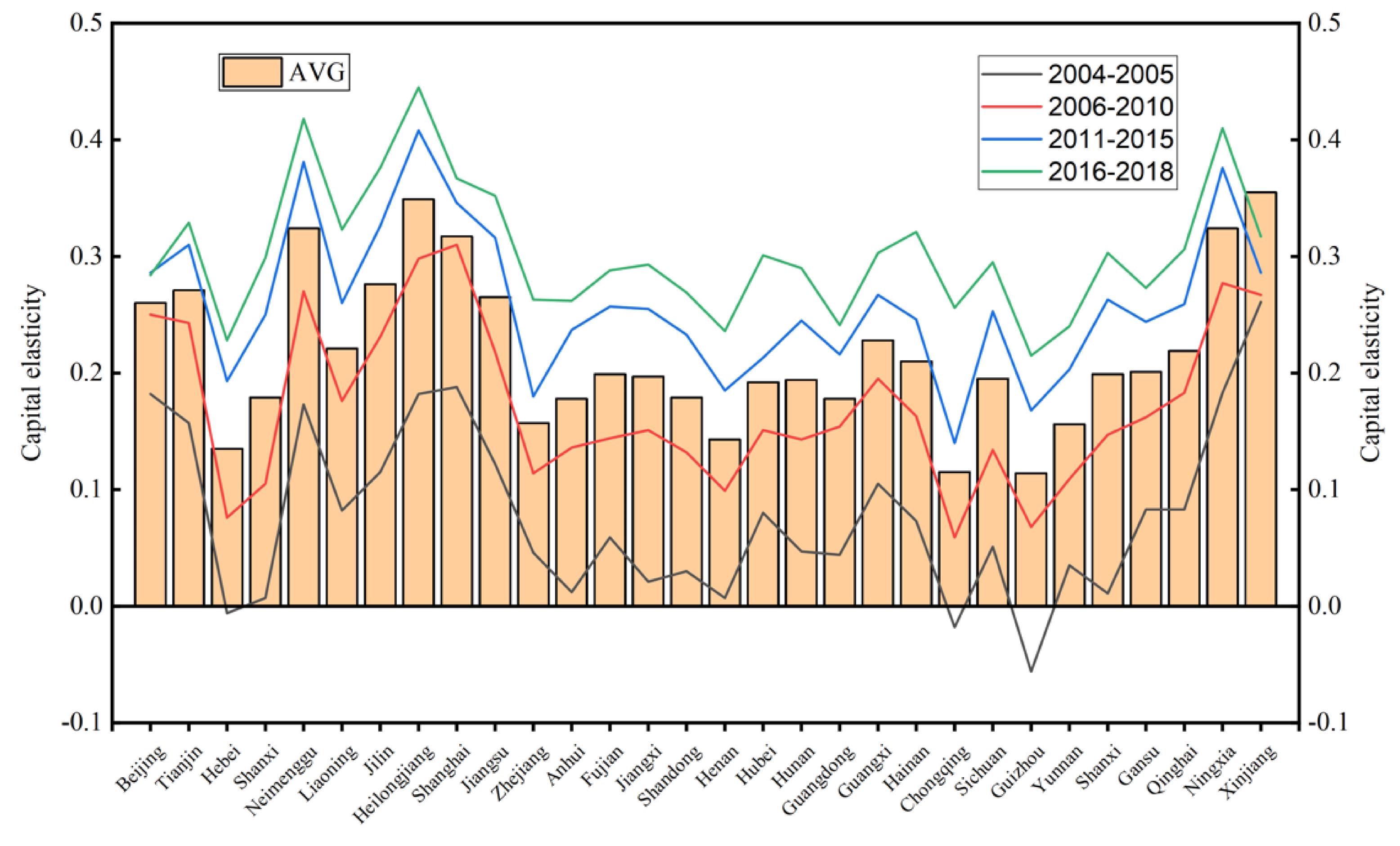
According to the output elasticity of capital of each province in China from 2004 to 2018 (Table 4), the overall output elasticity of capital factors was low, and some provinces even had a negative value. For example, in 2004–2005, the output elasticity of Hebei was −0.006, Chongqing was −0.018, and Guizhou was −0.056. In terms of the average value over the past 15 years, the output elasticity of capital was highest in Xinjiang (0.355), followed by Heilongjiang (0.349) and Ningxia (0.324); the lower provinces were Hebei (0.192) and Chongqing (0.115), and the lowest was Guizhou (0.114).
In China, the output elasticity of capital factors varied significantly in different periods (Figure 5). Among them, the output elasticity of 2004–2005 and 2006–2010 were lower than the average value of these 15 years. Then, from 2011–2015 and 2016–2018, outputs were generally higher than the national average. It could be seen that although the output elasticity of capital of each province was relatively low, it had a tendency to increase year by year.
3.5. The Output Elasticity of Water
It could be seen from the output elasticity of water of each province in China from 2004 to 2018 (Table 5), the overall output elasticity of water varied greatly, with some provinces high or low, while other provinces had a negative value. In terms of the average value over the past 15 years, the output elasticity of water was highest in Beijing (1.323), followed by Tianjin (1.218) and Shanghai (1.134); the lower provinces were Guangdong (−0.006) and Jiangsu (−0.032), and the lowest was Xinjiang (−0.132).
In China, the output elasticity of water was increasing in different time periods (Figure 6). Among them, the output elasticity of 2004–2005 and 2006–2010 were lower than the average value of these 15 years. Then, from 2011–2015 and 2016–2018, outputs were generally higher than the national average.
3.6. Substitution Elasticity of Capital and Water
According to the substitution elasticity of capital and water of each province in China from 2004 to 2018 (Table 6), the overall substitution elasticity of capital and water varied greatly, with some provinces high or low, and other provinces had a more negative value. In terms of the average value over the past 15 years, the substitution elasticity was highest in Ningxia (3.603), followed by Shaanxi (2.377), and the lowest was Xinjiang (−14.356).
3.7. Comparison between National and Northeast Level
It could be seen from the technical efficiency, capital and water output elasticity, and total output elasticity of the nation and Northeast over the past 15 years, from 2004 to 2018 (Table 7), that the levels were different. Among them, the national technical efficiency level was lower than that of the Northeast, and the total output elasticity was roughly the same. Meanwhile, the technical efficiency declined, while the relative variability increased year by year in China.
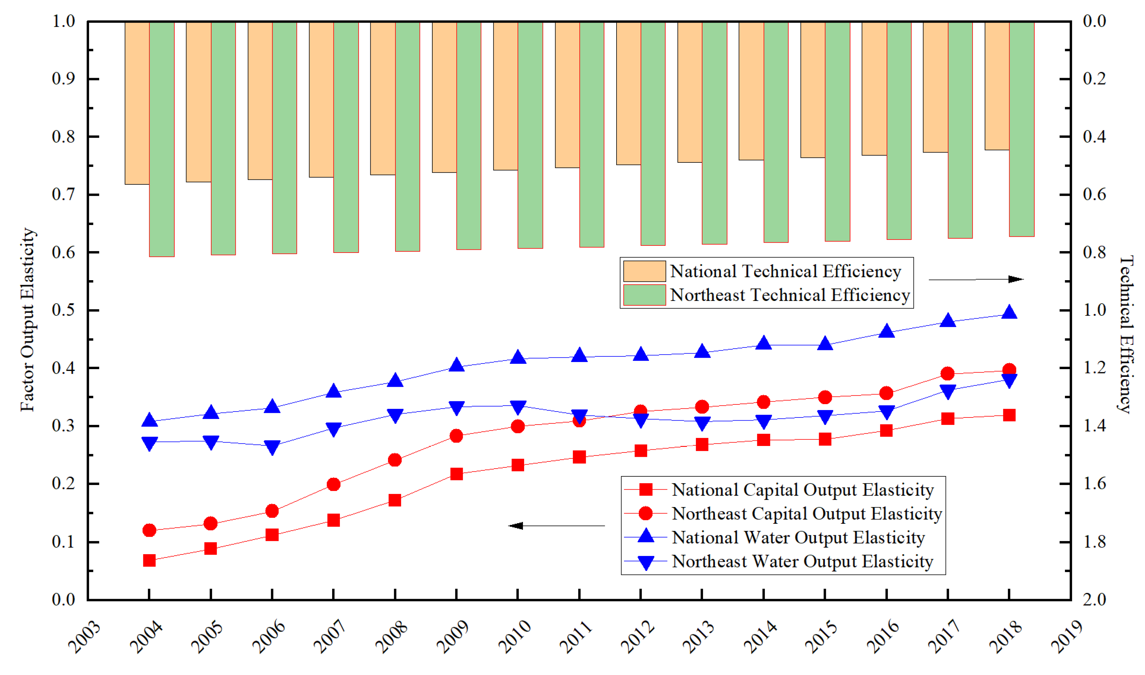
The technical efficiency of the nation and Northeast declined year by year, although the downward trend was not obvious (Figure 7). In terms of the output elasticity of capital, both the nation and Northeast were gradually rising, but the Northeast was higher than the nation. As for the output elasticity of water, the nation was on the rise and was higher than the Northeast, while in the Northeast, it was going up first, then falling, and finally rising again.
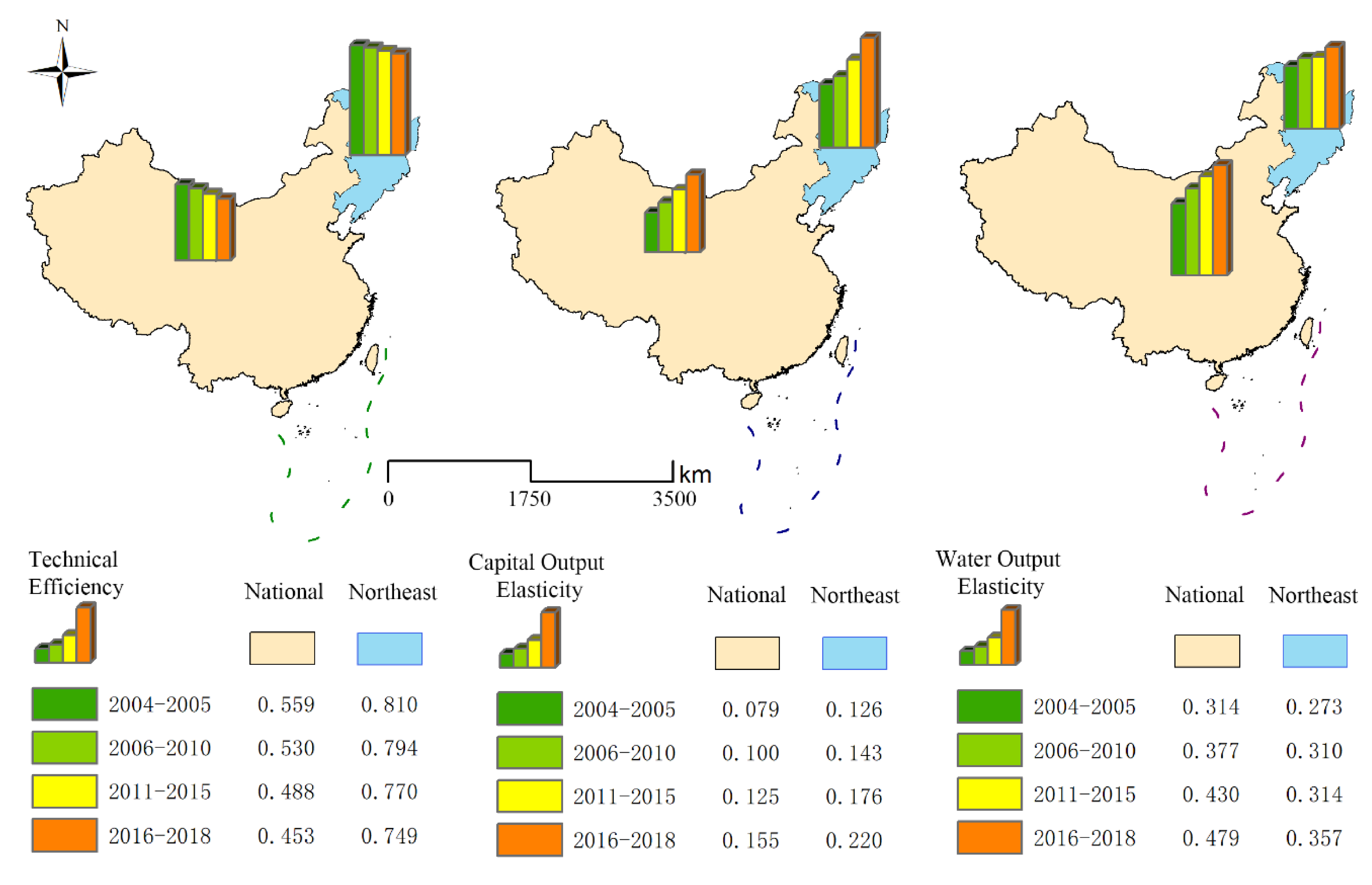
By comparing four different time periods (Figure 8), the technical efficiency of the nation and Northeast were the highest from 2004–2005, with 0.559 and 0.810, respectively. The output elasticity of capital was the highest in 2016–2018, with 0.155 and 0.220, respectively. Similarly, the output elasticity of water was also the highest in 2016–2018, with 0.479 and 0.357, respectively. At the same time, it was found that the technical efficiency of the nation and Northeast decreased year by year, while the output elasticity of capital and water increased year by year. However, the output elasticity of capital in the Northeast was higher than that of in the nation, but the output elasticity of water was the opposite.
4. Discussion
4.1. The Impact of Various Input Factors on Grain Production
From the perspective of technical efficiency, it was not necessarily the developed areas that have high technical efficiency of grain production, which was related to different input factors, especially the obvious difference of soil and water resources endowment in different regions [70,71]. In particular, there were fertile black soils and abundant water resources in Heilongjiang and Jilin, so the technical efficiency level was significantly higher than in other regions. After all, the Northeast was the birthplace of black soil in China [72], which was also concluded from the comparison between the nation and Northeast. At the same time, the overall level of technical efficiency was low in China, indicating that there was still tremendous room for the improvement of potential grain production.
From the perspective of output elasticity, the effect of the input of labor on grain production was not significant. At the same time, the output elasticity of capital was far less than the output elasticity of water, which meant that the input of water was increased in each additional percentage, and the power of output was far greater than that of the same amount of capital. It was indicated that the input structure of factors in grain production was seriously uncoordinated. Adjusting the structure of inputs was an important problem for the potential growth of food in the future. Meanwhile, water pollution adversely affected grain yield and agricultural production, which reduced the technical efficiency [73]. However, the amount of capital input used for chemical fertilizer and machinery purchase increased, and it would also play a key role in the improvement of agricultural production technologies, such as water-saving irrigation and water–fertilizer integration technologies [74]. The elasticity of capital output would increase year by year [75]. Therefore, it is necessary to strengthen expertise in agricultural science and technology to provide adequate financial support for agricultural research [76].
In addition, the output elasticity of capital and water was negative in many different regions. On the one hand, the application of agricultural production technology and modern machinery replaced the contribution of traditional rural labor to grain production [77]. To a certain extent, this could explain the phenomenon that food output was rising after labor transfer; on the other hand, there was still a large amount of surplus capital and water resources in some rural areas [78], and the marginal production of the capital or water was zero or even negative, which would also lead to an increase in capital or water resources and a decrease in grain production. It could be seen from the above that an increased investment in capital, labor, and water was not better. Only by reasonably controlling the appropriate amount of input to develop grain production could we achieve the maximum benefits. Therefore, when we adjust the structure of factor input, we should not only adjust measures to local conditions, but also distribute them reasonably to achieve the maximum output with minimum input and ensure the optimal allocation of existing resources.
4.2. Potential Risks of Water Resources
In the growth of food output, the output elasticity of water was higher than that of capital. Compared with the input of capital and labor, agricultural water resources still occupied an irreplaceable main position [79]. This conclusion was consistent with the current mainstream view in China. From the perspective of substitution elasticity, the value of most regions was greater than zero, which indicated that the input of water did play a decisive role in the increase of grain production capacity, while the substitution elasticity was less than zero. It also showed that water and capital in these regions are complementary, and they are a kind of synergy.
On the whole, the average technical efficiency of China showed a decreasing trend year by year, while the relative degree of variation was increasing slowly, indicating that the development frequency of soil and water resources was too high year by year and the demand for water resources was increasing. The fragility of land was increasing, which led to the risk of water resources shortage. The gradual decline of technical efficiency in the Northeast could also be verified, which was related to the decline of food productivity caused by the annual loss of black soil, soil acidification, and hardening [80,81]. Therefore, we must primarily protect water resources.
4.3. Strategies and Implications
For agriculture in the new era, we must improve quality and efficiency, optimize the input structure of various elements reasonably, protect the water ecological environment, and realize the high-quality development of grain production. In particular, modern intelligent agriculture, scientific planting, and highly mechanized operations have increasing advantages, and the requirements for the quality of labor are also higher. In the past, the role of the number of laborers to enhance the value of agricultural output has been gradually reduced or even disappeared. Therefore, we should increase the investment in education and training of rural labor, establish and improve the long-term mechanism of education and training, strengthen the efficient combination of theory and practice ability, and cultivate new farmers with higher quality skills, so that the “active” production factor of rural labor can be coupled and coordinated with other agricultural production factors. At the same time, as regions are affected by Covid-19 and natural disasters, it is a question of balance to get enough food nutrition and maintain ecologically friendly practices in grain production, sustainability, and the vulnerable areas, especially in the rural markets acting for vulnerable empowerment and grain growth [82]. Grain production is seriously affected by climate extremes, which are becoming more frequent and more severe under climate change, and food security will be consequently confronted with increasing risks. The increasing demand for grain production has resulted in the use of large quantities of water and other resources. There is an urgent need for innovative methods and approaches to augment the limited water and resources for enough grain production to guarantee the vulnerable groups of the poor and women have food security. However, knowledge gaps exist in this area that need to be addressed. A good mechanism for management of grain production could have an effective role in appealing to vulnerable populations. After all, agriculture is an essential livelihood option for most rural markets, so it is foremost for rural development.
Based on the empirical analysis of the technical efficiency, output elasticity, and substitution elasticity of agricultural production factors, this paper has the following policy implications: First, we should accelerate the pace of balanced allocation of agricultural production factors. Especially for water allocation, solutions should be tailored to local conditions, not only considering the natural resource endowments of each province, but also on the basis of technical efficiency and output elasticity. For example, the water resource was insufficient in Beijing and Shanghai, but the output elasticity of water was high, so it is necessary to consider water diversion to increase the amount of water. Heilongjiang was rich in water and had high technical efficiency, the status quo could be kept. For Xinjiang, the water was sufficient, but the output elasticity of water was very low and the technical efficiency was not high. Therefore, water allocation should be reduced or controlled. More attention should be paid to the improvement of agricultural production technology, the treatment of agricultural water pollution, and the efforts to cultivate high-quality application-oriented experts in agriculture. Second, we will strengthen the protection of water resources and cultivated land. With the rapid development of the economy and the deterioration of the ecological environment, the protection of water resources is extremely urgent [83]. The red line of ecology and arable land area must be ensured so as to protect the input of high-quality water and soil resources for the sustainable production of food. Third, we should vigorously promote the progress of agricultural technology, constantly invent and innovate crop cultivation technology, improve seed for farming technology [84], and increase agricultural intermediate investments to extend the agricultural industry chain, improve agricultural technical efficiency, and accelerate the development of agricultural modernization.
5. Conclusions
In this paper, the SFA model combined with the grain production function was used to study the technical efficiency and the output elasticity of grain production in China from 2004 to 2018. However, at present, most scholars have considered the efficiency of conventional resources rather than the most important factors of the input of water in grain production and these studies also do not provide much attention to in the value of output elasticity, so this paper holds particular significance. Furthermore, the SFA model is a more reliable method to calculate efficiency and elasticity, but the traditional DEA model cannot effectively deal with the problem of output elasticity and the SFA model makes up for this defect to some extent. Therefore, there is some innovation in the method presented in this paper. The results showed that: (1) The water resource was insufficient in Beijing and Shanghai, but the output elasticity of water was high, and Heilongjiang was rich in water and had high technical efficiency. For Xinjiang, the water was sufficient, but the output elasticity of water was very low and the technical efficiency was not high. Adjusting the structure of input factors was an essential measure for the potential growth of food in the future. (2) The overall level of technical efficiency of grain production in China was relatively low and still declining year by year. The output elasticity of water was far greater than that of capital, so we still need to explore the potentiality of grain production. (3) If the water resources increased by 3.94%, the grain yield increased by 10.46% and the yield had reached the maximum. Finally, we need to optimize the input structure of various elements, carry out the relevant policies to protect water resources, and realize the high-quality development of grain production. Also, the demand for food and increasing food accessibility have soared during the time of personal and mobility restrictions due to the impact of Covid-19 and natural disasters [85]. In the future of our work, the sustainability of grain production and supply worldwide urgently needs to be improved to protect water resources and human well-being. Therefore, corporate social responsibility has become a part of core agri-food operations, which create shared value for society. By integrating SFA models and comparing between the nation and Northeast in a novel approach, this study makes the important contribution to the field of taking water into account for decision making, and indicates a new direction for water resource allocation and management.
Author Contributions
Conceptualization, S.Y., H.W., and J.T.; methodology and software, S.Y., J.M. and F.Z.; investigation, F.Z. and J.M.; formal analysis, S.W.; writing—original draft, S.Y.; supervision, H.W.; writing—review and editing, H.W. and J.T. All authors have read and agreed to the published version of the manuscript.
Funding
This research was funded by National Key Research and Development Program of China (Grant No. 2017YFC0404600), International Cooperation and Exchange of the National Natural Science Foundation of China (Grant No. 51861125101), National Social Science Fund (Grant No. 15BGL128) and Fundamental Research Funds for the Central Universities (Grant No. KYCX20_0509).
Conflicts of Interest
The authors declare no conflict of interest.
References
- FAO. The Future of Food and Agriculture—Trends and Challenges; FAO: Roma, Italy, 2017. [Google Scholar]
- Ibrahiem, D.M.; Hanafy, S.A. Dynamic linkages amongst ecological footprints, fossil fuel energy consumption and globalization: An empirical analysis. Manag. Environ. Qual. Int. J. 2020. [Google Scholar] [CrossRef]
- Aivazidou, E.; Tsolakis, N.; Vlachos, D.; Iakovou, E. A water footprint management framework for supply chains under green market behaviour. J. Clean. Prod. 2018, 197, 592–606. [Google Scholar] [CrossRef]
- Arnold, M.G. Corporate social responsibility representation of the German water-supply and distribution companies: From colourful to barren landscapes. Int. J. Innov. Sustain. Dev. 2017, 11, 1–22. [Google Scholar] [CrossRef]
- Scarpato, D.; Civero, G.; Rusciano, V.; Risitano, M. Sustainable strategies and corporate social responsibility in the Italian fisheries companies. Corp. Soc. Responsib. Environ. Manag. 2020, 10, 1–8. [Google Scholar] [CrossRef]
- Jiao, X.; Lyu, Y.; Wu, X.; Li, H.; Cheng, L.; Zhang, C.; Yuan, L.; Jiang, R.; Jiang, B.; Rengel, Z. Grain production versus resource and environmental costs: Towards increasing sustainability of nutrient use in China. J. Exp. Bot. 2016, 67, 4935–4949. [Google Scholar] [CrossRef]
- Pingali, P.L. Green revolution: Impacts, limits, and the path ahead. Proc. Natl. Acad. Sci. USA 2012, 109, 12302–12308. [Google Scholar] [CrossRef] [Green Version]
- Kusch-Brandt, S. Towards More Sustainable Food Systems-14 Lessons Learned. Int. J. Environ. Res. Public Health 2020, 17, 4005. [Google Scholar] [CrossRef]
- Zhang, S.; Liu, Y.; Huang, D.-H. Contribution of factor structure change to China’s economic growth: Evidence from the time-varying elastic production function model. Econ. Res. Ekon. Istraživanja 2019, 1–24. [Google Scholar] [CrossRef] [Green Version]
- Bian, Y.; Yang, F. Resource and environment efficiency analysis of provinces in China: A DEA approach based on Shannon’s entropy. Energy Policy 2010, 38, 1909–1917. [Google Scholar] [CrossRef]
- Feng, C.; Huang, J.-B.; Wang, M. Analysis of green total-factor productivity in China’s regional metal industry: A meta-frontier approach. Resour. Policy 2018, 58, 219–229. [Google Scholar] [CrossRef]
- Babenko, A.; Vasilyeva, O. Factors of labour productivity growth in agriculture of the agrarian region. Balt. J. Econ. Stud. 2017, 3, 1–6. [Google Scholar] [CrossRef] [Green Version]
- Ustaoglu, E.; Castillo, C.P.; Jacobs-Crisioni, C.; Lavalle, C. Economic evaluation of agricultural land to assess land use changes. Land Use Policy 2016, 56, 125–146. [Google Scholar] [CrossRef]
- Artuzo, F.D.; Foguesatto, C.R.; da Silva, L.X. Precision Agriculture: Innovation for world food production and to optimization in the use of fertilizers. Rev. Tecnol. E Soc. 2017, 13, 146–160. [Google Scholar]
- Sun, X.; Wu, G.; Ren, X. The impact of chemical fertilizer input changes on grain production efficiency—An empirical analysis based on panel data of counties in Guizhou Province. J. South. Agric. 2019, 50, 1869–1877. [Google Scholar]
- Tapia Zurita, M.; Tapia Zurita, E. The Andean markets and their requirements for agricultural machinery. 3C Empresa 2017, 6, 47–62. [Google Scholar] [CrossRef] [Green Version]
- Jiang, M.; Li, X.; Xin, L.; Tan, M. The impact of paddy rice multiple cropping index changes in Southern China on national grain production capacity and its policy implications. Acta Geogr. Sin. 2019, 74, 32–43. [Google Scholar]
- Li, Z.; Jun, Z. Study on the estimation of agricultural production efficiency in Shandong province based on DEA-Malmquist model. Hubei Agric. Sci. 2019, 58, 219. [Google Scholar]
- Shi, C.; Zhan, P.; Zhu, J. Land Transfer, Factor Allocation and Agricultural Production Efficiency Improvement. China Land Sci. 2020, 34, 49–57. [Google Scholar]
- Shi, Z.; Huang, H.; Wu, Y.; Chiu, Y.H.; Qin, S. Climate Change Impacts on Agricultural Production and Crop Disaster Area in China. Int. J. Environ. Res. Public Health 2020, 17, 4792. [Google Scholar] [CrossRef]
- Lv, N.; Zhu, L. Study on China’s Agricultural Environmental Technical Efficiency and Green Total Factor Productivity Growth. J. Agrotech. Econ. 2019, 4, 95–103. [Google Scholar]
- Agovino, M.; Cerciello, M.; Gatto, A. Policy efficiency in the field of food sustainability. The adjusted food agriculture and nutrition index. J. Environ. Manag. 2018, 218, 220–233. [Google Scholar] [CrossRef] [PubMed]
- Le, T.L.; Lee, P.-P.; Peng, K.C.; Chung, R.H. Evaluation of total factor productivity and environmental efficiency of agriculture in nine East Asian countries. Agric. Econ. 2019, 65, 249–258. [Google Scholar]
- Vicente, J.R. Economic efficiency of agricultural production in Brazil. Rev. De Econ. E Sociol. Rural 2004, 42, 201–222. [Google Scholar] [CrossRef] [Green Version]
- Holden, S.; Shiferaw, B. Land degradation, drought and food security in a less-favoured area in the Ethiopian highlands: A bio-economic model with market imperfections. Agric. Econ. 2004, 30, 31–49. [Google Scholar] [CrossRef]
- Vollrath, D. Land distribution and international agricultural productivity. Am. J. Agric. Econ. 2007, 89, 202–216. [Google Scholar] [CrossRef]
- Abou-Ali, H.; El-Ayouti, A. Nile water pollution and technical efficiency of crop production in Egypt: An assessment using spatial and non-parametric modelling. Environ. Ecol. Stat. 2014, 21, 221–238. [Google Scholar] [CrossRef]
- Ogundari, K. Crop diversification and technical efficiency in food crop production. Int. J. Soc. Econ. 2013, 40, 267–288. [Google Scholar] [CrossRef]
- Devi, L.G.; Singh, Y.C. Resource use and technical efficiency of rice production in Manipur. Econ. Aff. 2014, 59, 823. [Google Scholar]
- Griliches, Z. Research expenditures, education, and the aggregate agricultural production function. Am. Econ. Rev. 1964, 54, 961–974. [Google Scholar]
- Yuize, Y. Nogyo ni okeru Kyoshiteki Seisan-kansu no Keisoku. Aggreg. Prod. Funct. Agric. Nogyo Sogo Kenkyu 1964, 18, 1–54. [Google Scholar]
- Lio, M.; Liu, M.-C. Governance and agricultural productivity: A cross-national analysis. Food Policy 2008, 33, 504–512. [Google Scholar] [CrossRef]
- Po-Chi, C.; Ming-Miin, Y.; Chang, C.-C.; Shih-Hsun, H. Total factor productivity growth in China’s agricultural sector. China Econ. Rev. 2008, 19, 580–593. [Google Scholar]
- Monchuk, D.C.; Chen, Z.; Bonaparte, Y. Explaining production inefficiency in China’s agriculture using data envelopment analysis and semi-parametric bootstrapping. China Econ. Rev. 2010, 21, 346–354. [Google Scholar] [CrossRef]
- Amaza, P.S.; Olayemi, J. Analysis of technical inefficiency in food crop production in Gombe State, Nigeria. Appl. Econ. Lett. 2002, 9, 51–54. [Google Scholar] [CrossRef]
- Latruffe*, L.; Balcombe, K.; Davidova, S.; Zawalinska, K. Determinants of technical efficiency of crop and livestock farms in Poland. Appl. Econ. Lett. 2004, 36, 1255–1263. [Google Scholar] [CrossRef]
- Min, R.; Gu, G. Empirical study on technical efficiency of grain production from the perspective of sustainable development—Observation based on panel data and sequence DEA of counties in Hubei Province. J. Hubei Univ. Philos. Soc. Sci. 2012, 39, 46–51. [Google Scholar] [CrossRef]
- Mareth, T.; Scavarda, L.F.; Thomé, A.M.T.; Oliveira, F.L.C.; Alves, T.W. Analysing the determinants of technical efficiency of dairy farms in Brazil. Int. J. Product. Perform. Manag. 2019, 68, 464–481. [Google Scholar] [CrossRef]
- Liu, Z.; Wang, C. Organic Agricultural Production Efficiency Based on a Three-stage DEA Model: A Case Study of Yang County, Shaanxi Province. Chin. J. Popul. Resour. Environ. 2015, 25, 105–112. [Google Scholar]
- Moutinho, V.; Madaleno, M.; Macedo, P.; Robaina, M.; Marques, C. Efficiency in the European agricultural sector: Environment and resources. Environ. Sci. Pollut. Res. 2018, 25, 17927–17941. [Google Scholar] [CrossRef]
- Feng, J.; Yang, J.; Jiang, H. Analysis of Grain Production Efficiency in the Major Grain Producing Counties of Jilin Province. J. Jilin Agric. Univ. 2015, 4, 493–498. [Google Scholar]
- Zhan-wei, L. On the Efficiency of Grain Production in the Undeveloped Areas—A Study Based on the DEA Method and Malmquist Index. J. Jiangxi Agric. Univ. 2011, 2, 9–15. [Google Scholar]
- Mwangi, T.M.; Ndirangu, S.N.; Isaboke, H.N. Technical efficiency in tomato production among smallholder farmers in Kirinyaga County, Kenya. Afr. J. Agric. Res. 2020, 16, 667–677. [Google Scholar]
- Fan, Q.; Dong, Z.; Du, F.; Chen, K. Application of stochastic frontier production function in the study of technical efficiency of grain production. Water Sav. Irrig. 2008, 6, 30–33. [Google Scholar]
- Tan, Z.; Guo, X. Evaluation and analysis of China’s grain production efficiency: Based on the super efficiency DEA model. Res. Agric. Mod. 2019, 3, 431–440. [Google Scholar]
- Dooley, D.M.; Griffiths, E.J.; Gosal, G.S.; Buttigieg, P.L.; Hoehndorf, R.; Lange, M.C.; Schriml, L.M.; Brinkman, F.S.; Hsiao, W.W. FoodOn: A harmonized food ontology to increase global food traceability, quality control and data integration. NPJ Sci. Food 2018, 2, 1–10. [Google Scholar] [CrossRef] [PubMed]
- Zhang, F.; Zhang, Q.; Li, F.; Fu, H.; Yang, X. Evaluation of grain production efficiency in the main production area based on the three stage DEA-WINDOWS. Chin. J. Agric. Resour. Reg. Plan 2019, 40, 158–165, 194. [Google Scholar]
- Wu, G.; Zhang, Q.; Zhang, F. Research on Grain Production Efficiency and Its Spatial Spillover Effects in China. Econ. Geogr. 2019, 9, 207–212. [Google Scholar]
- Wu, Y. Measurement of input-output elasticity of regional agricultural production factors in China—An empirical study based on spatial econometric model. Chin. Rural Econ. 2010, 6, 25–37. [Google Scholar]
- Yang, X.; Mu, Y. Irrigation water pressure, supply elasticity and grain production structure based on heterogeneous coefficient Nerlove model. J. Nat. Resour. 2020, 35, 728–742. [Google Scholar]
- Zhang, L.; Li, R. Research on Agricultural Machinery Service Development and Grain Production Efficiency: 2004–2016—Based on stochastic Frontier analysis of variable coefficients. J. Huazhong Agric. Univ. Soc. Sci. Ed. 2020, 2, 67–77. [Google Scholar]
- Liu, C.; Chen, X. Study on technical efficiency and influencing factors of grain production in China: Analysis of translog-SFA model based on interprovincial panel data. J. Chin. Agric. Mech. 2019, 40, 201–207. [Google Scholar]
- Hampf, B. Estimating emission coefficients and mass balances using economic data: A stochastic frontier approach. J. Ind. Ecol. 2019, 23, 932–945. [Google Scholar]
- Song, J.; Oh, D.-h.; Kang, J. Robust estimation in stochastic frontier models. Comput. Stat. Data Anal. 2017, 105, 243–267. [Google Scholar]
- Kumbhakar, S.C.; Lovell, C.K. Stochastic Frontier Analysis; Cambridge University Press: Cambridge, UK, 2003. [Google Scholar]
- Battese, G.E.; Coelli, T.J. Frontier production functions, technical efficiency and panel data: With application to paddy farmers in India. J. Product. Anal. 1992, 3, 153–169. [Google Scholar]
- Benedetti, I.; Branca, G.; Zucaro, R. Evaluating input use efficiency in agriculture through a stochastic frontier production: An application on a case study in Apulia (Italy). J. Clean. Prod. 2019, 236, 117609. [Google Scholar]
- Farrell, M.J. The measurement of productive efficiency. J. R. Stat. Soc. Ser. A 1957, 120, 253–281. [Google Scholar]
- Christensen, L.R.; Jorgenson, D.W.; Lau, L.J. Transcendental logarithmic production frontiers. Rev. Econ. Stat. 1973, 55, 28–45. [Google Scholar]
- Christensen, L.R.; Jorgenson, D.W.; Lau, L.J. Transcendental logarithmic utility functions. Am. Econ. Rev. 1975, 65, 367–383. [Google Scholar]
- Zhao, H.; Lin, B. Resources allocation and more efficient use of energy in China’s textile industry. Energy 2019, 185, 111–120. [Google Scholar]
- Cheng, Z.; Li, L.; Liu, J.; Zhang, H. Research on energy directed technical change in China’s industry and its optimization of energy consumption pattern. J. Environ. Manag. 2019, 250, 109471. [Google Scholar]
- Kutlu, L.; Tran, K.C.; Tsionas, M.G. A spatial stochastic frontier model with endogenous frontier and environmental variables. Eur. J. Oper. Res. 2020, 286, 389–399. [Google Scholar] [CrossRef]
- Jradi, S.; Parmeter, C.F.; Ruggiero, J. Quantile estimation of the stochastic frontier model. Econ. Lett. 2019, 182, 15–18. [Google Scholar] [CrossRef]
- Baggio, D.K.; Brizolla, M.M.B. Assessing Market Timing Performance of Brazilian Multi-Asset Pension Funds using the Battese and Coelli’s Stochastic Frontier Model (1995). Econ. Bull. 2020, 40, 50–60. [Google Scholar]
- Cechura, L.; Grau, A.; Hockmann, H.; Levkovych, I.; Kroupova, Z. Catching Up or Falling Behind in European Agriculture: The Case of Milk Production. J. Agric. Econ. 2017, 68, 206–227. [Google Scholar] [CrossRef]
- Coelli, T. Estimators and hypothesis tests for a stochastic frontier function: A Monte Carlo analysis. J. Product. Anal. 1995, 6, 247–268. [Google Scholar] [CrossRef]
- Hicks, J.R. Value and Capital: An Inquiry into Some Fundamental Principles of Economic Theory; Oxford University Press: New York, NY, USA, 1975. [Google Scholar]
- Drago, C.; Gatto, A. A robust approach to composite indicators exploiting interval data: The interval-valued global gender gap index (IGGGI). In Proceedings of IPAZIA Workshop on Gender Issues; Springer: Berlin/Heidelberg, Germany, 2018; pp. 103–114. [Google Scholar]
- WANG, Z.-F.; SU, X.; CHANG, H.-L. Water Resource Endowment and its Spatial Difference in China. J. Gansu Sci. 2007, 1, 145–148. [Google Scholar]
- Shepherd, K.D.; Soule, M.J. Soil fertility management in west Kenya: Dynamic simulation of productivity, profitability and sustainability at different resource endowment levels. Agric. Ecosyst. Environ. 1998, 71, 131–145. [Google Scholar] [CrossRef]
- Zhang, X.; Jiao, J. Formation and Evolution of Black Soil. J. Jilin Univ. (Earth Sci. Ed.) 2020, 2, 553–568. [Google Scholar]
- Tan, J.; Vila, J. Research on technical efficiency of grain production and its influencing factors—From panel data of 31 provinces in China from 1990 to 2013. J. Agrotech. Econ. 2016, 9, 72–83. [Google Scholar]
- Zhai, S.; Song, G.; Qin, Y.; Ye, X.; Lee, J. Modeling the impacts of climate change and technical progress on the wheat yield in inland China: An autoregressive distributed lag approach. PLoS ONE 2017, 12, e0184474. [Google Scholar] [CrossRef]
- Yan, J.; Zhang, Y.; Hua, X.; Yang, L. An explanation of labor migration and grain output growth: Findings of a case study in eastern Tibetan Plateau. J. Geogr. Sci. 2016, 26, 484–500. [Google Scholar] [CrossRef] [Green Version]
- Shi, Y.; Zhu, Y.; Wang, X.; Sun, X.; Ding, Y.; Cao, W.; Hu, Z. Progress and development on biological information of crop phenotype research applied to real-time variable-rate fertilization. Plant Methods 2020, 16, 11. [Google Scholar] [CrossRef] [PubMed]
- Shujun, L. Status and trends on sci-tech development of agricultural machinery in China. AMA Agric. Mech. Asia Afr. Lat. Am. 2016, 47, 115–120. [Google Scholar]
- Chen, K.; He, C.; Zhang, Y. The Migration of Surplus Labor and Technology Progress in China’s Agricultural Sector—The Theoretical Mechanism Based on Ranis-Fei Model and Micro Evidence from Eight Rural Villages in West China. Ind. Econ. Res. 2010, 1, 1–8. [Google Scholar]
- Kang, S.; Hao, X.; Du, T.; Tong, L.; Su, X.; Lu, H.; Li, X.; Huo, Z.; Li, S.; Ding, R. Improving agricultural water productivity to ensure food security in China under changing environment: From research to practice. Agric. Water Manag. 2017, 179, 5–17. [Google Scholar] [CrossRef]
- Shen, C.; Wang, Y.; Zhao, L.; Xu, X.; Yang, X.; Liu, X. Characteristics of material migration during soil erosion in sloped farmland in the black soil region of Northeast China. Trop. Conserv. Sci. 2019, 12, 1–11. [Google Scholar] [CrossRef] [Green Version]
- Xin, Y.; Liu, G.; Xie, Y.; Gao, Y.; Liu, B.; Shen, B. Effects of soil conservation practices on soil losses from slope farmland in northeastern China using runoff plot data. Catena 2019, 174, 417–424. [Google Scholar] [CrossRef]
- Gatto, A.; Polselli, N.; Bloom, G. Empowering gender equality through rural development: Rural markets and micro-finance in Kyrgyzstan. In L’europa E La Comunità Internazionale Difronte Alle Sfide Dello Svilupp; Giannini: Naples, Italy, 2016; pp. 65–89. [Google Scholar]
- Steinfeld, C.M.; Sharma, A.; Mehrotra, R.; Kingsford, R.T. The human dimension of water availability: Influence of management rules on water supply for irrigated agriculture and the environment. J. Hydrol. 2020, 588, 125009. [Google Scholar] [CrossRef]
- Wagan, S.A.; Memon, Q.U.A.; Yanwen, T. A comparison of input resource use and production efficiency of wheat between China and Pakistan using Stochastic Frontier Analysis (SFA). Custos E Agronegocio Line 2020, 16, 79–98. [Google Scholar]
- Cattivelli, V.; Rusciano, V. Social Innovation and Food Provisioning during Covid-19: The Case of Urban–Rural Initiatives in the Province of Naples. Sustainability 2020, 12, 4444. [Google Scholar] [CrossRef]
Figure 1.
Grain production in different provinces of China and the main producing areas (Northeast region).
Figure 1.
Grain production in different provinces of China and the main producing areas (Northeast region).

Figure 2.
Methodological framework applied in the present analysis.

Figure 3.
Grain production in different provinces, as well as capital, labor, and water inputs.

Figure 4.
Technical efficiency and average level in four different periods.

Figure 5.
The output elasticity of capital and average level in four different periods.

Figure 6.
The output elasticity of water and average level in four different periods.

Figure 7.
Comparison of technical efficiency and capital and water output elasticity between the nation and Northeast year by year.
Figure 7.
Comparison of technical efficiency and capital and water output elasticity between the nation and Northeast year by year.

Figure 8.
Comparison of technical efficiency and capital and water output elasticity between the nation and Northeast in four different time periods.
Figure 8.
Comparison of technical efficiency and capital and water output elasticity between the nation and Northeast in four different time periods.


Table 1.
Descriptive statistics.
| Variable | N | Minimum | Maximum | Mean | Standard Deviation |
|---|---|---|---|---|---|
| Grain () | 450 | 34.1400 | 7615.8000 | 1928.381227 | 1623.8381258 |
| Capital ( yuan) | 450 | 0.1122 | 46.6058 | 9.184820 | 9.0198438 |
| Labor ( people) | 450 | 205.0000 | 7045.2800 | 2417.289730 | 1685.1997177 |
| Water () | 450 | 4.2000 | 561.7500 | 123.504202 | 102.4522041 |
Table 2.
Cross-provincial stochastic frontier analysis (2004–2018), the results of MLE.
| Variable | Coefficient to Be Estimated | Value | Standard Deviation | t Test |
|---|---|---|---|---|
| Constant | −4.192053 | 2.838707 | −1.476747 | |
| 0.787380 | 0.185058 | 4.254774 *** | ||
| 0.915338 | 0.787451 | 1.162408 | ||
| 2.662388 | 0.838769 | 3.174161 *** | ||
| 0.070855 | 0.027508 | 2.575759 ** | ||
| 0.012049 | 0.148305 | 0.081247 | ||
| −0.338214 | 0.110734 | −3.054295 *** | ||
| −0.119321 | 0.025465 | −4.685656 *** | ||
| 0.046295 | 0.027361 | 1.691980 * | ||
| −0.111242 | 0.120526 | −0.922977 | ||
| 0.656665 | 0.293462 | 2.237647 ** | ||
| 0.840179 | 0.073301 | 11.462051 *** | ||
| 0.766576 | 0.361893 | 2.118242 ** | ||
| −0.028928 | 0.007408 | −3.904911 *** | ||
| Log Likelihood | −183.702090 *** | |||
| LR | 392.044620 *** | |||
Note: * means significant at the 10% level, ** at 5%, and *** at 1%. LR is the likelihood ratio statistic, which conforms to the mixed Chi-squared distribution.
Table 3.
The technical efficiency of 30 provinces in China (2004–2018).
| Province | 2004–2005 | 2006–2010 | 2011–2015 | 2016–2018 | AVG | Rank |
|---|---|---|---|---|---|---|
| Beijing | 0.649 | 0.620 | 0.576 | 0.538 | 0.593 | 11 |
| Tianjin | 0.811 | 0.793 | 0.766 | 0.741 | 0.776 | 5 |
| Hebei | 0.688 | 0.661 | 0.620 | 0.585 | 0.636 | 9 |
| Shanxi | 0.564 | 0.531 | 0.482 | 0.441 | 0.501 | 16 |
| Neimenggu | 0.696 | 0.669 | 0.629 | 0.595 | 0.644 | 8 |
| Liaoning | 0.587 | 0.554 | 0.506 | 0.466 | 0.525 | 14 |
| Jilin | 0.912 | 0.904 | 0.890 | 0.877 | 0.895 | 3 |
| Heilongjiang | 0.932 | 0.925 | 0.915 | 0.905 | 0.919 | 2 |
| Shanghai | 0.406 | 0.369 | 0.317 | 0.275 | 0.338 | 21 |
| Jiangsu | 0.649 | 0.620 | 0.576 | 0.539 | 0.593 | 10 |
| Zhejiang | 0.226 | 0.193 | 0.149 | 0.118 | 0.168 | 30 |
| Anhui | 0.697 | 0.670 | 0.630 | 0.596 | 0.646 | 7 |
| Fujian | 0.259 | 0.224 | 0.178 | 0.144 | 0.197 | 29 |
| Jiangxi | 0.557 | 0.523 | 0.473 | 0.432 | 0.493 | 17 |
| Shandong | 0.828 | 0.812 | 0.786 | 0.764 | 0.796 | 4 |
| Henan | 0.946 | 0.940 | 0.931 | 0.923 | 0.935 | 1 |
| Hubei | 0.575 | 0.542 | 0.493 | 0.452 | 0.512 | 15 |
| Hunan | 0.621 | 0.590 | 0.544 | 0.505 | 0.562 | 12 |
| Guangdong | 0.340 | 0.303 | 0.252 | 0.213 | 0.273 | 24 |
| Guangxi | 0.377 | 0.340 | 0.288 | 0.247 | 0.309 | 23 |
| Hainan | 0.286 | 0.251 | 0.202 | 0.166 | 0.222 | 28 |
| Chongqing | 0.782 | 0.762 | 0.731 | 0.703 | 0.742 | 6 |
| Sichuan | 0.594 | 0.562 | 0.514 | 0.474 | 0.533 | 13 |
| Guizhou | 0.504 | 0.468 | 0.417 | 0.374 | 0.437 | 19 |
| Yunnan | 0.510 | 0.475 | 0.423 | 0.381 | 0.444 | 18 |
| Shaanxi | 0.314 | 0.277 | 0.227 | 0.190 | 0.248 | 27 |
| Gansu | 0.403 | 0.366 | 0.313 | 0.272 | 0.335 | 22 |
| Qinghai | 0.330 | 0.293 | 0.243 | 0.204 | 0.263 | 25 |
| Ningxia | 0.408 | 0.371 | 0.318 | 0.276 | 0.339 | 20 |
| Xinjiang | 0.328 | 0.292 | 0.241 | 0.202 | 0.262 | 26 |
Table 4.
The output elasticity of capital of 30 provinces in China (2004–2018).
| Province | 2004–2005 | 2006–2010 | 2011–2015 | 2016–2018 | AVG | Rank |
|---|---|---|---|---|---|---|
| Beijing | 0.182 | 0.250 | 0.286 | 0.284 | 0.260 | 9 |
| Tianjin | 0.157 | 0.243 | 0.310 | 0.329 | 0.271 | 7 |
| Hebei | −0.006 | 0.076 | 0.193 | 0.228 | 0.135 | 28 |
| Shanxi | 0.007 | 0.105 | 0.250 | 0.299 | 0.179 | 22 |
| Neimenggu | 0.173 | 0.270 | 0.381 | 0.418 | 0.324 | 4 |
| Liaoning | 0.082 | 0.176 | 0.260 | 0.323 | 0.221 | 11 |
| Jilin | 0.115 | 0.231 | 0.326 | 0.376 | 0.276 | 6 |
| Heilongjiang | 0.182 | 0.298 | 0.408 | 0.445 | 0.349 | 2 |
| Shanghai | 0.188 | 0.310 | 0.346 | 0.367 | 0.317 | 5 |
| Jiangsu | 0.122 | 0.218 | 0.316 | 0.352 | 0.265 | 8 |
| Zhejiang | 0.046 | 0.114 | 0.180 | 0.263 | 0.157 | 25 |
| Anhui | 0.012 | 0.136 | 0.237 | 0.262 | 0.178 | 23 |
| Fujian | 0.059 | 0.144 | 0.257 | 0.288 | 0.199 | 15 |
| Jiangxi | 0.021 | 0.151 | 0.255 | 0.293 | 0.197 | 17 |
| Shandong | 0.030 | 0.132 | 0.233 | 0.269 | 0.179 | 21 |
| Henan | 0.007 | 0.099 | 0.185 | 0.236 | 0.143 | 27 |
| Hubei | 0.080 | 0.151 | 0.213 | 0.301 | 0.192 | 20 |
| Hunan | 0.047 | 0.143 | 0.245 | 0.290 | 0.194 | 19 |
| Guangdong | 0.044 | 0.154 | 0.216 | 0.241 | 0.178 | 24 |
| Guangxi | 0.105 | 0.195 | 0.267 | 0.303 | 0.228 | 10 |
| Hainan | 0.073 | 0.163 | 0.246 | 0.321 | 0.210 | 13 |
| Chongqing | −0.018 | 0.059 | 0.140 | 0.256 | 0.115 | 29 |
| Sichuan | 0.051 | 0.134 | 0.253 | 0.295 | 0.195 | 18 |
| Guizhou | −0.056 | 0.068 | 0.168 | 0.215 | 0.114 | 30 |
| Yunnan | 0.035 | 0.109 | 0.203 | 0.240 | 0.156 | 26 |
| Shaanxi | 0.011 | 0.147 | 0.263 | 0.303 | 0.199 | 16 |
| Gansu | 0.083 | 0.162 | 0.244 | 0.273 | 0.201 | 14 |
| Qinghai | 0.083 | 0.183 | 0.259 | 0.306 | 0.219 | 12 |
| Ningxia | 0.183 | 0.277 | 0.376 | 0.410 | 0.324 | 3 |
| Xinjiang | 0.261 | 0.267 | 0.286 | 0.317 | 0.355 | 1 |
Table 5.
The output elasticity of water of 30 provinces in China (2004–2018).
| Province | 2004–2005 | 2006–2010 | 2011–2015 | 2016–2018 | AVG | Rank |
|---|---|---|---|---|---|---|
| Beijing | 1.140 | 1.227 | 1.357 | 1.548 | 1.323 | 1 |
| Tianjin | 1.113 | 1.179 | 1.250 | 1.298 | 1.218 | 2 |
| Hebei | 0.015 | 0.072 | 0.176 | 0.242 | 0.133 | 24 |
| Shanxi | 0.608 | 0.654 | 0.674 | 0.694 | 0.662 | 7 |
| Neimenggu | 0.185 | 0.273 | 0.355 | 0.374 | 0.309 | 16 |
| Liaoning | 0.300 | 0.343 | 0.402 | 0.487 | 0.386 | 12 |
| Jilin | 0.435 | 0.489 | 0.473 | 0.505 | 0.479 | 11 |
| Heilongjiang | 0.086 | 0.099 | 0.067 | 0.079 | 0.082 | 25 |
| Shanghai | 0.999 | 1.123 | 1.171 | 1.182 | 1.134 | 3 |
| Jiangsu | −0.117 | −0.067 | −0.010 | 0.048 | −0.032 | 29 |
| Zhejiang | 0.182 | 0.257 | 0.334 | 0.448 | 0.311 | 15 |
| Anhui | 0.114 | 0.120 | 0.166 | 0.184 | 0.147 | 22 |
| Fujian | 0.227 | 0.299 | 0.394 | 0.448 | 0.351 | 14 |
| Jiangxi | 0.100 | 0.144 | 0.176 | 0.222 | 0.164 | 21 |
| Shandong | 0.014 | 0.077 | 0.178 | 0.237 | 0.134 | 23 |
| Henan | 0.097 | 0.124 | 0.189 | 0.248 | 0.167 | 20 |
| Hubei | 0.120 | 0.153 | 0.158 | 0.249 | 0.169 | 19 |
| Hunan | −0.056 | 0.028 | 0.098 | 0.128 | 0.060 | 27 |
| Guangdong | −0.125 | −0.022 | 0.022 | 0.051 | −0.006 | 28 |
| Guangxi | −0.036 | 0.049 | 0.099 | 0.139 | 0.072 | 26 |
| Hainan | 0.662 | 0.733 | 0.800 | 0.871 | 0.774 | 6 |
| Chongqing | 0.758 | 0.844 | 0.803 | 0.890 | 0.828 | 5 |
| Sichuan | 0.119 | 0.177 | 0.205 | 0.199 | 0.183 | 18 |
| Guizhou | 0.397 | 0.482 | 0.560 | 0.536 | 0.508 | 10 |
| Yunnan | 0.174 | 0.244 | 0.312 | 0.322 | 0.273 | 17 |
| Shaanxi | 0.449 | 0.502 | 0.576 | 0.605 | 0.540 | 9 |
| Gansu | 0.271 | 0.328 | 0.378 | 0.414 | 0.354 | 13 |
| Qinghai | 0.877 | 0.934 | 0.978 | 1.063 | 0.967 | 4 |
| Ningxia | 0.505 | 0.586 | 0.677 | 0.740 | 0.637 | 8 |
| Xinjiang | −0.179 | −0.146 | −0.126 | −0.089 | −0.132 | 30 |
Table 6.
The substitution elasticity of capital and water of 30 provinces in China (2004–2018).
| Province | 2004–2005 | 2006–2010 | 2011–2015 | 2016–2018 | AVG |
|---|---|---|---|---|---|
| Beijing | 1.117 | 1.134 | 1.124 | 1.094 | 1.120 |
| Tianjin | 1.109 | 1.141 | 1.161 | 1.158 | 1.147 |
| Hebei | 1.241 | 0.006 | 0.039 | −0.039 | 0.172 |
| Shanxi | 1.091 | 1.237 | 1.685 | 1.946 | 1.509 |
| Neimenggu | −0.034 | −0.011 | 0.059 | 0.094 | 0.030 |
| Liaoning | 2.821 | −1.475 | −1.156 | −1.556 | −0.812 |
| Jilin | 1.734 | 9.742 | −1.205 | −0.771 | 2.923 |
| Heilongjiang | 0.111 | 0.156 | 0.138 | 0.157 | 0.144 |
| Shanghai | 1.157 | 1.207 | 1.216 | 1.229 | 1.208 |
| Jiangsu | 1.906 | −0.450 | −0.043 | 0.108 | 0.111 |
| Zhejiang | −0.478 | 0.499 | −2.121 | −3.685 | −1.341 |
| Anhui | 4.764 | −0.062 | 0.113 | 0.127 | 0.678 |
| Fujian | 5.094 | −2.242 | −1.069 | −1.626 | −0.750 |
| Jiangxi | 0.983 | −0.052 | 0.126 | 0.126 | 0.181 |
| Shandong | 0.020 | 0.063 | 0.101 | 0.068 | 0.071 |
| Henan | 6.298 | −0.135 | −0.025 | −0.034 | 0.780 |
| Hubei | −0.178 | −0.020 | 0.094 | 0.099 | 0.021 |
| Hunan | −2.233 | 0.024 | 0.141 | 0.166 | −0.209 |
| Guangdong | 2.142 | −0.097 | 0.054 | 0.103 | 0.292 |
| Guangxi | −0.175 | 0.059 | 0.148 | 0.173 | 0.080 |
| Hainan | 1.164 | 1.271 | 1.372 | 1.451 | 1.326 |
| Chongqing | 1.052 | 1.099 | 1.189 | 1.293 | 1.162 |
| Sichuan | −0.586 | −0.220 | 0.085 | 0.149 | −0.093 |
| Guizhou | 0.997 | 1.297 | 1.618 | 2.364 | 1.578 |
| Yunnan | 9.477 | −4.281 | −0.767 | −0.381 | −0.496 |
| Shaanxi | 1.155 | 1.748 | 2.830 | 3.487 | 2.377 |
| Gansu | 4.777 | −1.010 | −1.051 | −1.126 | −0.275 |
| Qinghai | 1.109 | 1.178 | 1.233 | 1.234 | 1.198 |
| Ningxia | 2.136 | 3.294 | 4.613 | 3.414 | 3.603 |
| Xinjiang | −77.817 | −10.592 | −1.050 | −0.500 | −14.356 |
Table 7.
Comparison between national and northeast levels (2004–2018).
| Year | Technical Efficiency | Capital Output Elasticity | Water Output Elasticity | Total Output Elasticity | Standard Deviation | Relative Variability | ||||
|---|---|---|---|---|---|---|---|---|---|---|
| Nation | Northeast | Nation | Northeast | Nation | Northeast | Nation | Northeast | Nation | Nation | |
| 2004 | 0.563 | 0.813 | 0.069 | 0.12 | 0.308 | 0.273 | 0.377 | 0.393 | 0.205 | 0.364 |
| 2005 | 0.555 | 0.808 | 0.089 | 0.132 | 0.321 | 0.274 | 0.41 | 0.406 | 0.207 | 0.373 |
| 2006 | 0.547 | 0.804 | 0.112 | 0.153 | 0.331 | 0.266 | 0.443 | 0.419 | 0.21 | 0.384 |
| 2007 | 0.539 | 0.799 | 0.138 | 0.199 | 0.358 | 0.297 | 0.496 | 0.496 | 0.212 | 0.394 |
| 2008 | 0.53 | 0.795 | 0.172 | 0.241 | 0.376 | 0.32 | 0.548 | 0.561 | 0.214 | 0.405 |
| 2009 | 0.522 | 0.79 | 0.218 | 0.283 | 0.403 | 0.334 | 0.621 | 0.617 | 0.217 | 0.415 |
| 2010 | 0.513 | 0.785 | 0.232 | 0.299 | 0.416 | 0.335 | 0.648 | 0.634 | 0.219 | 0.426 |
| 2011 | 0.505 | 0.78 | 0.247 | 0.309 | 0.42 | 0.319 | 0.667 | 0.628 | 0.221 | 0.438 |
| 2012 | 0.496 | 0.775 | 0.258 | 0.325 | 0.421 | 0.313 | 0.679 | 0.638 | 0.223 | 0.45 |
| 2013 | 0.488 | 0.77 | 0.268 | 0.333 | 0.426 | 0.308 | 0.694 | 0.641 | 0.225 | 0.461 |
| 2014 | 0.479 | 0.765 | 0.276 | 0.341 | 0.441 | 0.311 | 0.717 | 0.652 | 0.227 | 0.474 |
| 2015 | 0.47 | 0.76 | 0.277 | 0.35 | 0.44 | 0.318 | 0.717 | 0.668 | 0.229 | 0.486 |
| 2016 | 0.462 | 0.755 | 0.292 | 0.357 | 0.462 | 0.327 | 0.754 | 0.684 | 0.23 | 0.499 |
| 2017 | 0.453 | 0.749 | 0.313 | 0.39 | 0.48 | 0.362 | 0.793 | 0.752 | 0.232 | 0.512 |
| 2018 | 0.445 | 0.744 | 0.319 | 0.397 | 0.494 | 0.381 | 0.813 | 0.778 | 0.234 | 0.525 |
© 2020 by the authors. Licensee MDPI, Basel, Switzerland. This article is an open access article distributed under the terms and conditions of the Creative Commons Attribution (CC BY) license (http://creativecommons.org/licenses/by/4.0/).
Share and Cite
MDPI and ACS Style
Yang, S.; Wang, H.; Tong, J.; Ma, J.; Zhang, F.; Wu, S. Technical Efficiency of China’s Agriculture and Output Elasticity of Factors Based on Water Resources Utilization. Water 2020, 12, 2691. https://doi.org/10.3390/w12102691
AMA Style
Yang S, Wang H, Tong J, Ma J, Zhang F, Wu S. Technical Efficiency of China’s Agriculture and Output Elasticity of Factors Based on Water Resources Utilization. Water. 2020; 12(10):2691. https://doi.org/10.3390/w12102691
Chicago/Turabian StyleYang, Shiliang, Huimin Wang, Jinping Tong, Jianfeng Ma, Fan Zhang, and Shijuan Wu. 2020. "Technical Efficiency of China’s Agriculture and Output Elasticity of Factors Based on Water Resources Utilization" Water 12, no. 10: 2691. https://doi.org/10.3390/w12102691
Note that from the first issue of 2016, this journal uses article numbers instead of page numbers. See further details here.