Introduction of Confidence Interval Based on Probability Limit Method Test into Non-Stationary Hydrological Frequency Analysis

Abstract

Nonstationarity in hydrological variables has been identified throughout Japan in recent years. As a result, the reliability of designs derived from using method based on the assumption of stationary might deteriorate. Non-stationary hydrological frequency analysis is among the measures to counter this possibility. Using this method, time variations in the probable hydrological quantity can be estimated using a non-stationary extreme value distribution model with time as an explanatory variable. In this study, we build a new method for constructing the confidence interval regarding the non-stationary extreme value distribution by applying a theory of probability limit method test. Furthermore, by introducing a confidence interval based on probability limit method test into the non-stationary hydrological frequency analysis, uncertainty in design rainfall because of lack of observation information was quantified, and it is shown that assessment pertaining to both the occurrence risk of extremely heavy rainfall and changes in the trend of extreme rainfall accompanied with climate change is possible.

1. Introduction

Design rainfall, the reference value in flood control measures, is determined by performing a probability-based statistical analysis termed hydrological frequency analysis [1] on observed data of maximum rainfall in the past. Traditional hydrological frequency analyses assume a stationary hydrological quantity. This steadiness implies that the probability law influencing hydrological quantity does not change in time. In other words, traditional methods often use the concept that the probability distribution which hydrological quantities are assumed to follow does not change in time. However, in recent years, increasingly non-stationary hydrological quantity has been identified, ascribed to the effects of climate change associated with global warming [2,3,4,5]. In this context, this unsteadiness implies either that the time series of hydrological quantity has both a trend and cycle, or that the probability distribution followed by hydrological quantity changes temporally. In Japan, it is predicted that the amount of rainfall and the frequency of floods will increase in the future because of climate change. A report highlighting such predictions was published by the National Institute for Land and Infrastructure Management [6]. In this report, it was shown to be possible for the amount of rainfall during the design rainfall duration time in main river basins to increase 1.1- to 1.3-fold nationwide. Therefore, considering that rainfall is intensified as a result of the climate change described above, it is urgent to develop statistical methods that consider the unsteadiness of the hydrological quantity in order to draw up flood control measures.

In recent years, numerous studies and reports have noted the non-stationarity of the hydrological quantity. For example, Milly et al. [7] challenged the assumption of stationarity in the field of hydrology in the perspective of the effects of the climate change and stated that a non-stationary probability distribution of hydrological quantity should be considered when defining planning and management. Sado et al. [8] analyzed time series of annual maximum daily precipitation in the Hokkaido region considering the jump of mean and dispersion and investigated the unsteadiness of the probable hydrological quantity. Additionally, Sogawa et al. [9] investigated the unsteadiness of the annual maximum daily precipitation in various parts of Japan and clarified the period length (sample size) during which unsteadiness could be definitely confirmed. Also, Yamada et.al [10] investigated a number of annual maximum precipitation records in Japan, and incorporated the influence of the long-term temperature trend into sampling theory [11,12]. As a result, they showed the existence of increasing trend of temperature by comparison between actual observed new records which is enumerated from the beginning of observation and theoretical number of new records derived from the sampling theory considering the effect of temperature change. Based on their previous researches, hydrological frequency analysis should be conducted considering non-stationarity of rainfall. From the perspective of actual frequency analysis for nonstationary probable rainfall, Kitano et al. [13] expanded the concept of the degree of experience [14] showing a theory that reflected the durability of observation information in estimated values of probable rainfall to evaluate its change in the future.

Non-stationary hydrological frequency analysis is a statistical method able to consider non-stationarity in hydrological quantity. Traditional hydrological frequency analysis methods have been developed based on the extreme value theory by Fisher and Tippet [15]. They theoretically derived a function form of the extreme value distribution, which is the probability distribution that the maximum value in a sample follows. Later, Gumbel [16] adopted their extreme value distribution as the probability distribution of flood discharge and performed a pioneer study of hydrological frequency analysis. The extreme value distribution is classified into three types of functional forms depending on its positive or negative parameter, i.e., Gumbel distribution, Frechet distribution, and negative Weibull distribution. Gnedenko [17] demonstrated a necessary and sufficient condition for the probability distribution belonging to the domain of attraction of the extreme value distribution. Mises [18] and Jenkinson [19] expressed the above-mentioned three types of extreme value distribution as one functional form, and this is used as a generalized extreme value distribution. In addition, for a specific non-stationary hydrological frequency analysis, Coles [20] showed a non-stationary extreme value distribution model by expressing the parameter of non-stationary extreme value distribution as poly-nomial with time as an explanatory variable and showed its applications (in the present paper, this parameter is also described as time-varying parameter). Khaliq [21] summarized non-stationary hydrological frequency analysis methods and theories. Furthermore, El Adlouni [22] demonstrated improved methods for the estimation of the parameters of the non-stationary extreme value distribution model. Towler [23] used the non-stationary generalized extreme value distribution model as the probability distribution of river discharge, applying it to future predictions of water quality. In addition, Hayashi et al. [24] showed analytically that AIC (Aakaike Information Criteria [25]) and TIC (Takeuchi Information Criteria [26]) were effective as model selection criteria for the non-stationary extreme value distribution model. Here, AIC are model selection criteria which are the approximated asymptotic bias of TIC with numbers of free parameters. These model selection criteria are applied to observed data at nationwide weather agency stations and GCM (Global Climate Model) output data of the Meteorological Research Institute in Japan, in order to clarify future changes in annual maximum daily precipitation.

Nonetheless, hydrological frequency analysis is deficient because of the lack of observed extremes such as annual maximum rainfall, since the observation period of rainfall is limited; therefore, it experiences difficulty arising from the fact that uncertainty is mostly included in probable rainfall. Among the resulting negative effects are that the observed data of record-breaking heavy rainfall significantly deviate from the adopted probability distribution and, if a return period of heavy rainfall is evaluated based on a traditional hydrological frequency analysis, its return period becomes several thousand or tens of thousands of years. Since flood control measures for major rivers in Japan are generally formulated with a design return period of approximately 100 to 200 years, a method to reasonably evaluate record-breaking heavy rainfalls using traditional hydrological frequency analysis is yet to be established; therefore, these heavy rainfall may be treated as “beyond the scope of assumption.” A concept exists to contribute to resolving such a difficulty: “confidence interval.” Interval estimation is among the statistical estimation methods that uses a sample X when estimating unknown parameter θ in a population distribution by construction of the lower confidence limit, L_C.I.(X), and upper confidence limit, U_C.I.(X), and that subsequently guarantees that parameter θ is contained within the interval of these confidence limits, [L_C.I.(X), U_C.I.(X)] with a probability of (1 − p) or greater, where, p is the significance level certifying the probability that the parameter θ is not contained in the confidence interval. In such cases, the interval [L_C.I.(X), U_C.I.(X)] is termed as the confidence interval and has a confidence coefficient of 1 − p or 100 × (1 − p)% [27]. By introducing the confidence interval, the range that T-year rainfall takes can be theoretically estimated. This in turn makes it possible to understand the probability distribution based on the observation of past records, which was adopted by traditional methods, as like an expected value of the distribution. In addition, it also becomes possible to estimate the swing of T-year probability hydrological quantities in flood control measures for a T-year probability scale. This makes it possible to interpret the record-breaking heavy rainfall mentioned above as a phenomenon within the confidence interval. In other words, the confidence interval enables a rational evaluation of return period of heavy rainfall.

Nowadays, in Japan, flood risk assessment is performed by utilizing a confidence interval based on a downscaled large ensemble climate projection database d4PDF [28,29,30]. d4PDF [31,32] contains numerous calculated rainfall data for past and future climate. Such database can be interpreted as rainfall data which we could have possibly experienced in the past and might experience with some probability in the future. Yamada et al. [28,29,30] conducted downscaling simulations of the ensemble climate projection database d4PDF and constructed a horizontal high-resolution data of resolution high enough to evaluate future rainfall characteristics and proposed an application of the downscaled database into flood control management. Also, Shimizu et al. [33,34,35] showed a method to determine the confidence interval using the theory of the probability limit method test, as created by Moriguti [36]. In previous researches, confidence intervals are often expressed by numerical methods such as the jackknife or bootstrap method [37]. Many of these conventional methods use an assumption of normality to estimate statistics. On the other hands, confidence interval based on probability limit method test does not require any parametric assumptions as possible. In addition, the occurrence risk that the upper confidence limit line value, which can be corresponded to extremely heavy rainfall can be obtained from the product of “target return period” and “one-sided probability of the confidence interval” [33,34,35]. Also, the confidence interval resulting from probability limit method test corresponds closely to the confidence interval using the sample group consisted of a downscaled large ensemble climate projection database constructed by Yamada et al. [28,29,30,35]. This result verifies downscaling simulations from the theoretical perspective and suggests that the risk of extremely heavy rainfall, which might be treated as beyond the scope of assumption in the past, can be included in flood control management. As a summary, the novelty of the proposed confidence interval [35] is that it can quantify uncertainty of design level rainfall, which is caused by the shortage of extreme rainfall data. In addition, from the consistency of confidence interval based on the theory and downscaling simulations [35], outliers which cannot be handled in traditional framework are interpreted as values at right tail of distribution of probable rainfall, and given occurrence probability to realize clarified interpretation for outliers.

In this study, the confidence interval of the non-stationary extreme value distribution was constructed by applying probability limit method test theory to the non-stationary hydrological frequency analysis. Through introducing the confidence interval into non-stationary hydrological frequency analysis, the assessment of the risk of extremely heavy rainfall considering changes in the trend of the extreme hydrological quantities associated with climate change becomes possible. The details of this finding are enumerated in the following.

2. Overview of Target Data

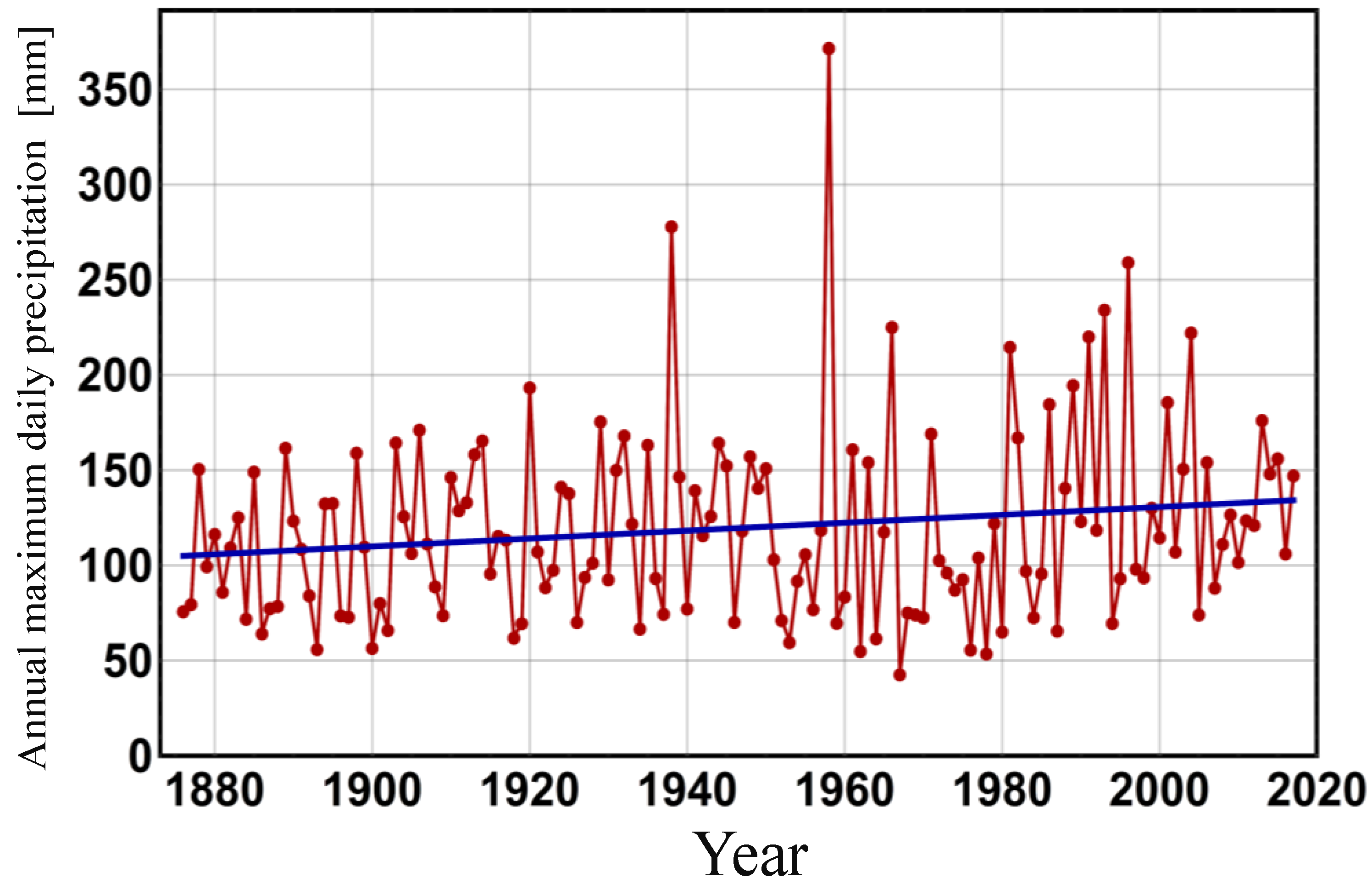
In this chapter, the abstract of the data used for the non-stationary hydrological frequency analysis is shown. The target data are observed data for annual maximum daily precipitation over 142 years from 1876 to 2017 at the Meteorological Agency ground observation station Tokyo. Time series of these observed data are shown in Figure 1. The maximum in the time series shown in Figure 1 is 371.9 mm occurring by the influence of Kanogawa Typhoon (Typhoon Ida), which occurred in 1958. To understand the characteristics of this time series data, a linear model assuming time as the explanatory variable was applied to the data in order to obtain a regression line, which is shown as a blue solid line in Figure 1. The slope of this regression line indicates an increasing trend of the annual maximum daily precipitation at the observation station. It is also possible to confirm the increasing trend in the annual maximum daily precipitation by visual observation without using the regression line. For example, an increasing trend in the annual maximum daily precipitation in recent years is visible in Figure 1 when the behaviors of the time series of observed data for approximately 40 years from 1876 (the starting year of observations) and those of from 1980 to 2017 are compared.

Thus, it was confirmed that a more rational probability hydrological quantity could be estimated by applying the non-stationary hydrological frequency analysis to the data.

3. Overview of the Non-Stationary Extreme Value Distribution Model

In this chapter, the non-stationary Gumbel distribution and non-stationary generalized extreme value distribution are introduced as examples of the non-stationary extreme value distribution models, and their abstracts are presented. Hereafter, the cumulative distribution function, probability density function, and probability representing function of the non-stationary extreme value distributions mentioned above are expressed as F_X(x, t), f_X(x, t), and χ_X(u, t), respectively. The probability representing function is an inverse function of the cumulative distribution function [38].

In the following, the function forms of both distribution models are shown, where t is time, μ(t) is a location parameter, σ(t) is a scale parameter, and ξ(t) is a shape parameter.

(1)

Non-stationary Gumbel distribution model:

$$f_X\left(x,t\right)=\frac{1}{\sigma \left(t\right)}\exp \left[-\left(\frac{x-\mu \left(t\right)}{\sigma \left(t\right)}\right)\right] \exp \left[-\exp \left\{-\left(\frac{x-\mu \left(t\right)}{\sigma \left(t\right)}\right)\right\}\right]$$

(1)

$$F_X\left(x,t\right)=\exp \left[-\exp \left\{-\left(\frac{x-\mu \left(t\right)}{\sigma \left(t\right)}\right)\right\}\right]$$

(2)

$${\chi }_X\left(u,t\right)=\mu \left(t\right)-\sigma \left(t\right)\log \left[-\log \left(u\right)\right]$$

(3)

(2)

Non-stationary generalized extreme value distribution model:

$$f_X\left(x,t\right)=\frac{1}{\sigma \left(t\right)}\exp \left[-{\left(1+\frac{\xi \left(t\right)\left(x-\mu \left(t\right)\right)}{\sigma \left(t\right)}\right)}^{-\frac{1}{\xi \left(t\right)}}\right] {\left(1+\frac{\xi \left(t\right)\left(x-\mu \left(t\right)\right)}{\sigma \left(t\right)}\right)}^{-1-\frac{1}{\xi \left(t\right)}}$$

(4)

$$F_X\left(x,t\right)=\exp \left[-{\left(1+\frac{\xi \left(t\right)\left(x-\mu \left(t\right)\right)}{\sigma \left(t\right)}\right)}^{-\frac{1}{\xi \left(t\right)}}\right]$$

(5)

$${\chi }_X\left(u,t\right)=\mu \left(t\right)-\frac{\sigma \left(t\right)\left(1-{\left(-\log \left(u\right)\right)}^{-\xi \left(t\right)}\right)}{\xi \left(t\right)}$$

(6)

where ξ(t) ≠ 0, 1 + ξ(t) (x − μ(t))/σ(t) > 0. Note that, when shape parameter ξ(t) = 0, the non-stationary generalized extreme value distribution model corresponds to the non-stationary Gumbel distribution model.

The parameter of the non-stationary extreme value distribution model is expressed by a function with the time as an explanatory variable. Here, the shape parameter, ξ(t), is often treated as a constant, assuming that it does not change over time for practical reasons.

$$\mu \left(t\right)={\displaystyle \sum _{k = 0}^q{\mu }_k{t}^k}$$

(7)

$$\sigma \left(t\right)=\exp \left({\displaystyle \sum _{k = 0}^r{\sigma }_k{t}^k}\right)$$

(8)

$$\xi \left(t\right)=\xi$$

(9)

where q and r are the highest degree of the location parameter μ(t) and the scale parameter σ(t), respectively.

Note that when parameter estimation is performed with the maximum likelihood method, the time t is discretized as shown below.

$$t_i=\frac{i}{n+1}, \left(i=1,2,\cdots ,n,\cdots \right)$$

(10)

where t_i is the discretized time, i is the number of years (I = 1, 2, …, n), and n is the number of observation years. Note that when the annual maximum series data are treated, n corresponds to the total number of observed data.

The maximum likelihood method is a parameter estimation method assuming a value of the parameter that maximizes a likelihood function L(θ) shown in Equation (11) to be its estimated value, where time series data are expressed as {x₁, x₂, …, x_n} and parameter vectors are expressed as θ.

$$L\left(\theta \right)={\displaystyle \prod _{i = 1}^n{f}_X\left(x_i, t_i\right)}$$

(11)

4. Application of the Non-Stationary Extreme Value Distribution Model to the Target Data

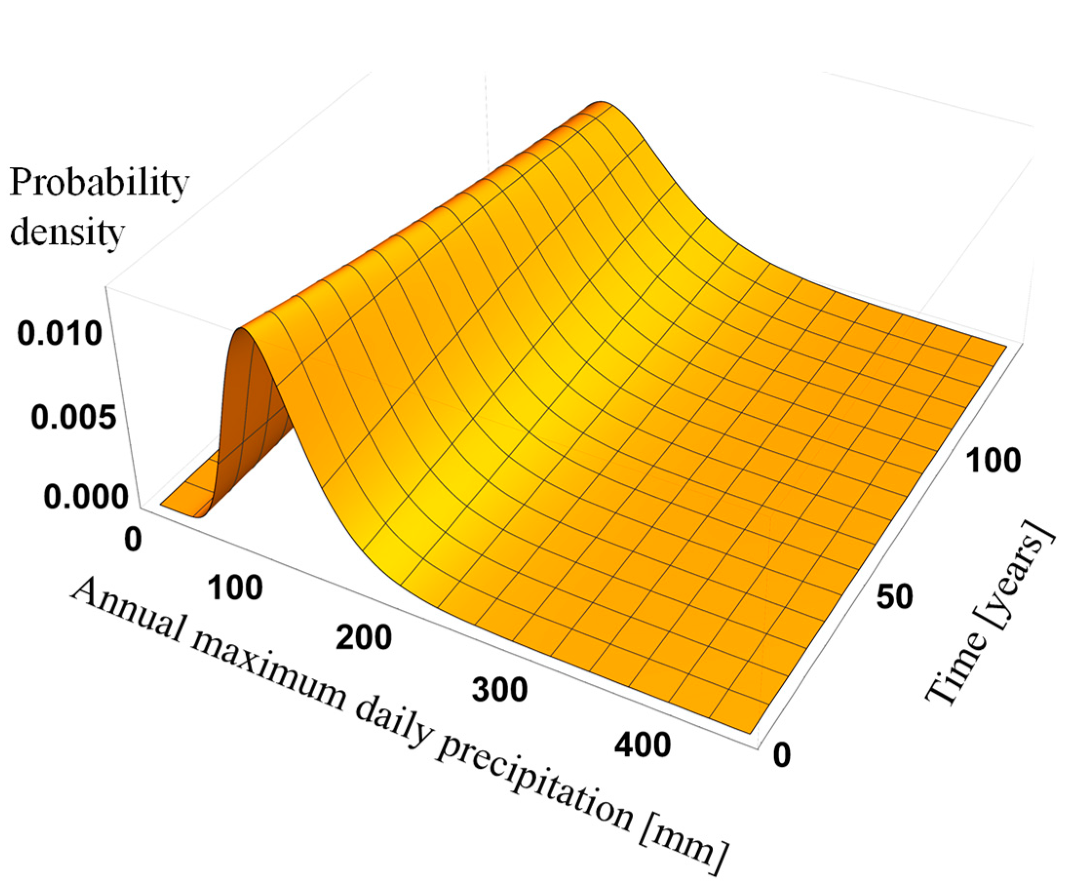
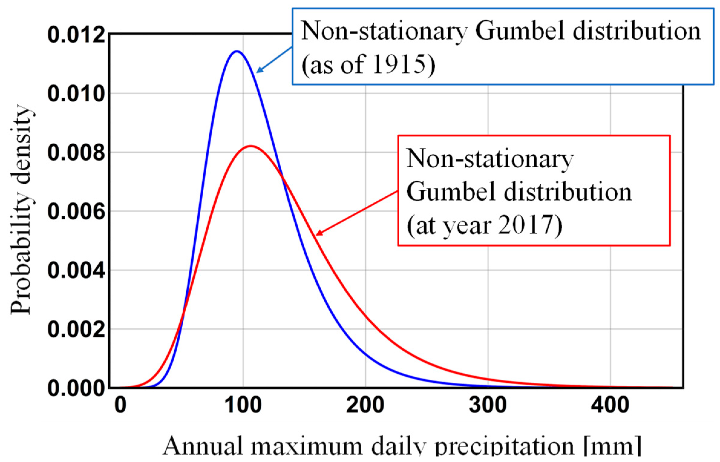
In this study, the non-stationary Gumbel distribution was adopted for frequency analysis. In this chapter, an abstract of the non-stationary Gumbel distribution applied to the target data is presented. Figure 2 shows the probability density function of the non-stationary Gumbel distribution applied to the observed data of annual maximum daily precipitation over 142 years (from 1876 to 2017) at the ground observation station Tokyo. Figure 2 indicates that the probability density function of the non-stationary Gumbel distribution underwent change with time. Note that the highest degree of the time-varying parameter was set at 1 for both the location parameter and scale parameter. The following equations are the functional forms of these time-varying parameters. Figure 3 shows the non-stationary Gumbel distribution applied to target data from 1915 and 2017. The blue solid line represents the non-stationary Gumbel distribution for 1915, whereas the red solid line represents the non-stationary Gumbel distribution for 2017. From Figure 2 and Figure 3, it is found that the right tail of the non-stationary Gumbel distribution expands and the mode value increases with proceeding of time. This indicates that the increasing trend of annual maximum daily precipitation is reflected in the estimated non-stationary Gumbel distribution.

$$\mu \left(t\right)={\mu }_0+{\mu }_{1}t$$

(12)

$$\sigma \left(t\right)=\exp \left({\sigma }_0+{\sigma }_{1}t\right)$$

(13)

5. Methodology

This chapter shows a methodology to construct the confidence interval of non-stationary extreme value distribution based on probability limit method test [36] for evaluation of extremely heavy rainfall in future period. Probability limit method test is a hypothesis test theory to improve the issues inherent to the Kolmogorov-Smirnov test [39,40] such that test power is weak at both tails of the assumed probability distribution. Using this test, an acceptance region in a standard uniform distribution is obtained by utilizing a characteristic that an order statistic generated by the standard uniform distribution follows the beta distribution; then, the acceptance region in standard uniform distribution is converted to the acceptance region of observed ith order statistics using the probability distribution, which the actual observed data are assumed to follow. Here acceptance region is defined as a range constructed by critical values in both sides of an assumed probability distribution.

5.1. Calculation of Probability Limit Value in the Standard Uniform Distribution

Function forms of the cumulative distribution function, F_X(x, t), and the probability representing function, χ_X(u, t), of the non-stationary extreme value distribution fitted to the observed data are expressed using Equations (14) and (15), respectively,

$$u=F_X\left(x,t\right)$$

(14)

$$x={\chi }_X\left(u,t\right)$$

(15)

where x is the realized value of random variable X, t is time [year], and u is the cumulative probability (realized value of random variable U).

Based on probability limit method test, critical values are calculated in the standard uniform distribution (uniform distribution of interval [0,1]). Moriguti [36] defined the upper limit and the lower limit of the critical values in the standard uniform distribution as z_U(i) and z_L(i), respectively. In this paper, z_U(i) and z_L(i) are also referred to as the upper and lower probability limit values, respectively, and they are critical values in the standard uniform distribution. The cumulative probability U from an arbitrary continuous probability distribution is known to follow a standard uniform distribution. This holds true commonly for stationary and non-stationary probability distributions. In addition, the order statistic U_(i) derived from the standard uniform distribution follows a beta distribution in terms of parameter (i, n − i + 1). This is represented by Equation (16):

$$\begin{array}{cc}\hfill F_{U\left(i\right)}\left(i\right)& =P\left(U_{\left(i\right)}\le u\right)\hfill \\ \hfill & =I_u\left(i,n-i+1\right)\hfill \end{array}$$

(16)

where F_U(i) (u) is the cumulative distribution function of the ith order statistic U_(i), I_u (i, n − i + 1) is the cumulative distribution function of the beta distribution with parameter (i, n − i + 1), n is sample size (total number of observed data), and i is the rank order from smallest to largest.

To calculate the probability limit value in the standard uniform distribution, the occurrence probability of datum that deviates from the standard uniform distribution is expressed as “α_min,” which is sampled using a trial shown in Equation (17):

$${\alpha }_{\min }=\underset{1 \le i \le n}{\min }\left\{Min{\left[\begin{array}{c}{I}_u\left(i,n-i+1\right)\\ I_{1-u}\left(n-i+1, i\right)\end{array}\right]}_{u = u_{(i)}}\right\}$$

(17)

where I_u(i, n − i + 1)|_{u = u(i)} is the non-exceedance probability of the ith order statistic u_(i) following beta distribution with parameter (i, n − i + 1), and I_1-u (n − i + 1, i)|_{u = u(i)} is the exceedance probability of the ith order statistic u_(i) following beta distribution with parameter (i, n − i + 1).

By repeating the trial shown in Equation (17), the arbitrary number of α_min can be obtained. To make it easier to treat these data, α_min is transformed to a logarithm form, −log₁₀(2α_min). The distribution of −log₁₀(2α_min) can be regarded as the distribution of the occurrence probability of the order statistic that significantly deviates from the standard uniform distribution in the samples.

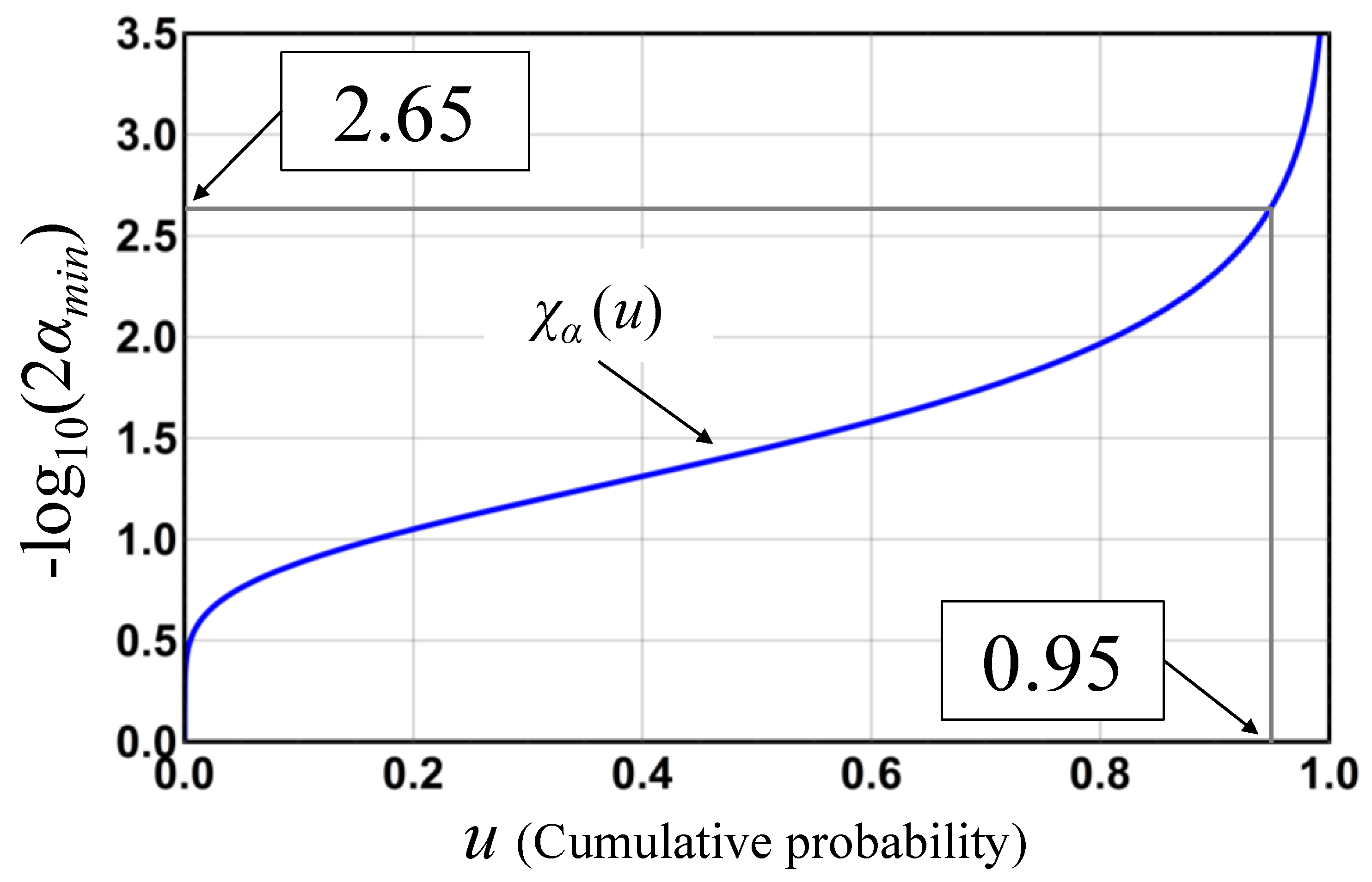
Shimizu et al. [33,34,35] proposed to fit the extreme value distribution to the sample of −log₁₀(2α_min) on the ground that −log₁₀(2α_min) becomes the maximum of the sample constructed from smaller value of the non-exceedance probability or the exceedance probability of the ith order statistic u_(i), which are transformed to the logarithm form in a similar way. By doing so, the probability limit value modified according to an arbitrary level of significance can be calculated. Figure 4 shows the probability representing function χ_α(u) of the Gumbel distribution that was fitted to the sample of −log₁₀(2α_min).

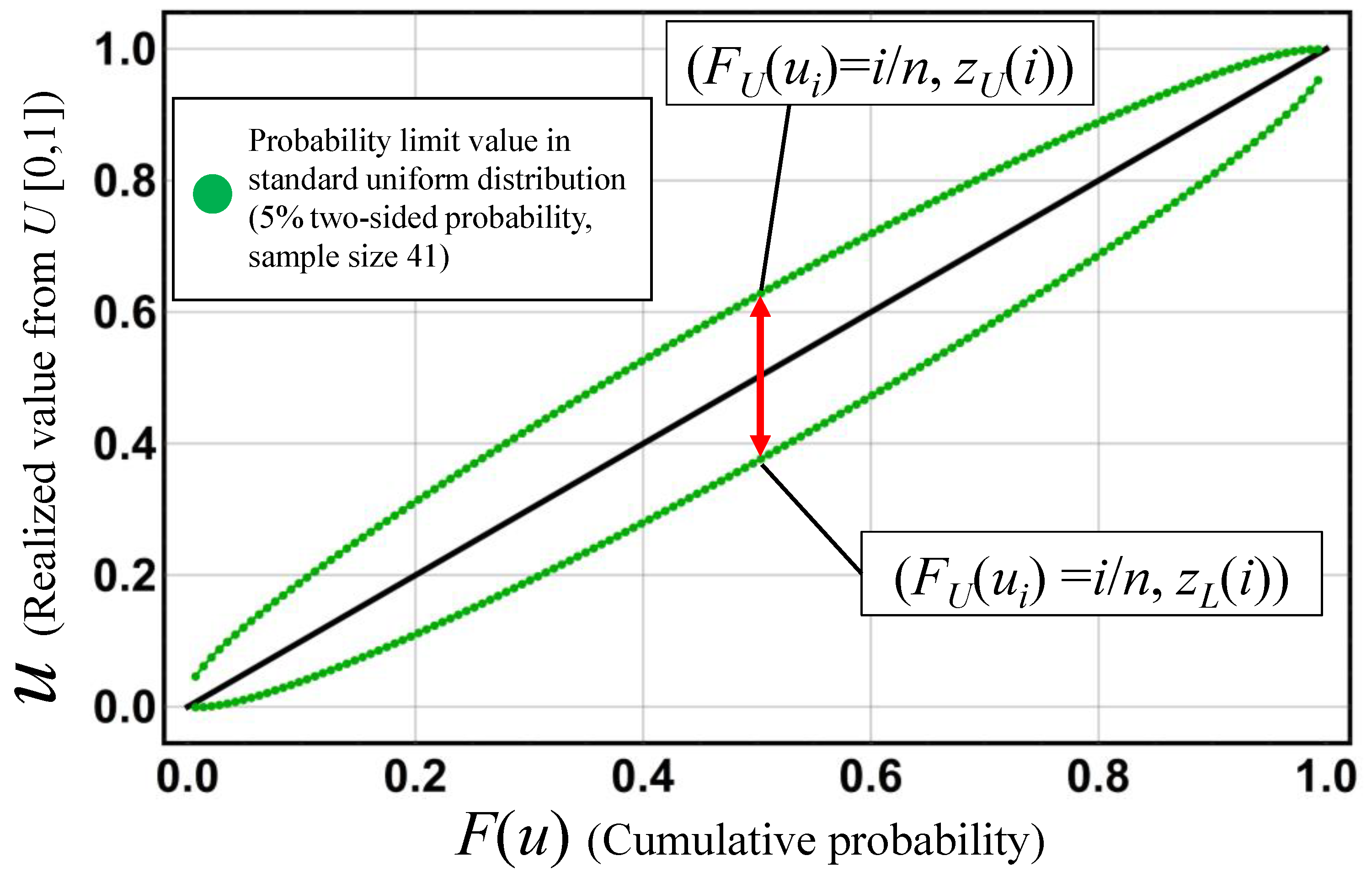
When probability limit method test is performed on target data assuming a probability distribution with a 5% significance level (5% two-sided probability), the value of α corresponding to this significance level (two-sided probability) is 1.12 × 10⁻³ after solving equation χ_α(0.95) = −log₁₀(2α_min) = 2.65 for α_min (refer to Figure 4 for each value in the equation). When the probability shown in Equation (16) is α, u becomes z_L(i), and when this probability becomes (1 − α), u becomes z_U(i). Since the sample size of the target data was 142, the sample of the upper probability limit value U_U is {z_U(1), z_U(2), …, z_U(142)}, whereas that of the lower probability limit value U_L is {z_L(1), z_L(2), …, z_L(142)}. Experimental points determined by providing these probability limit values with the cumulative probability, F_U(u_(i)), derived from a plotting position equation, are defined as the lower probability limit point (F_U(u_(i)), z_L(i)) and upper probability limit point (F_U(u_(i)), z_U(i)). In this case, the line interpolating (F_U(u_(i)), z_L(i)) is termed as the lower probability limit line, while that interpolating (F_U(u_i), z_U(i)) is termed the upper probability limit line. Figure 5 shows the probability limit lines of the standard uniform distribution with 5% two-sided probability and sample size 142. The area between both limit lines is the acceptance region based on probability limit method test for standard uniform distribution data.

5.2. Calculation of the Probability Limit Value in the Non-Stationary Extreme Value Distribution and Construction of the Confidence Interval

The probability limit value of the non-stationary extreme value distribution can be calculated by treating the probability limit value in standard uniform distribution as the cumulative probability and substituting it into the probability representing function of the non-stationary extreme value distribution at a given time t. The upper and lower probability limit values of the non-stationary extreme value distribution fitted to observed data are χ_X(z_U(i), t) and χ_X(z_L(i), t), respectively. In addition, the samples of the upper probability limit value, X_U, and the lower probability limit value, X_L, in the non-stationary extreme value distribution fitted to the observed data are defined as {χ_X(z_U(1), t), χ_X(z_U(2), t), …, χ_X(z_U(n), t)} and {χ_X(z_L(1), t), χ_X(z_L(2), t), …, χ_X(z_L(n), t)}, respectively, where n is the total number of the observed data.

Next, a process to construct the confidence interval of the non-stationary extreme value distribution at an arbitrary time t is shown. First, samples of the lower and upper probability limit values, X_L and X_U, respectively, are calculated for the target time t. Then, these samples are fitted to the stationary extreme value distribution corresponding to the adopted non-stationary extreme value distribution, and a parameter of its stationary extreme value distribution is estimated. For example, when the non-stationary Gumbel distribution (/the non-stationary generalized extreme value distribution) was adopted for fitting to the observed data, the Gumbel distribution (/the generalized extreme value distribution) was used for fitting to the probability limit values. Since the probability limit values are calculated with the assumption that the time t is given, the stationary probability limit value distribution is appropriate for fitting the probability limit values. In this study, the adopted stationary extreme value distribution with parameters estimated from samples X_U and X_L are defined as the upper confidence limit line and the lower confidence limit line, respectively. Therefore, the interval between both confidence limit lines is the confidence interval of the non-stationary extreme value distribution at the target time t.

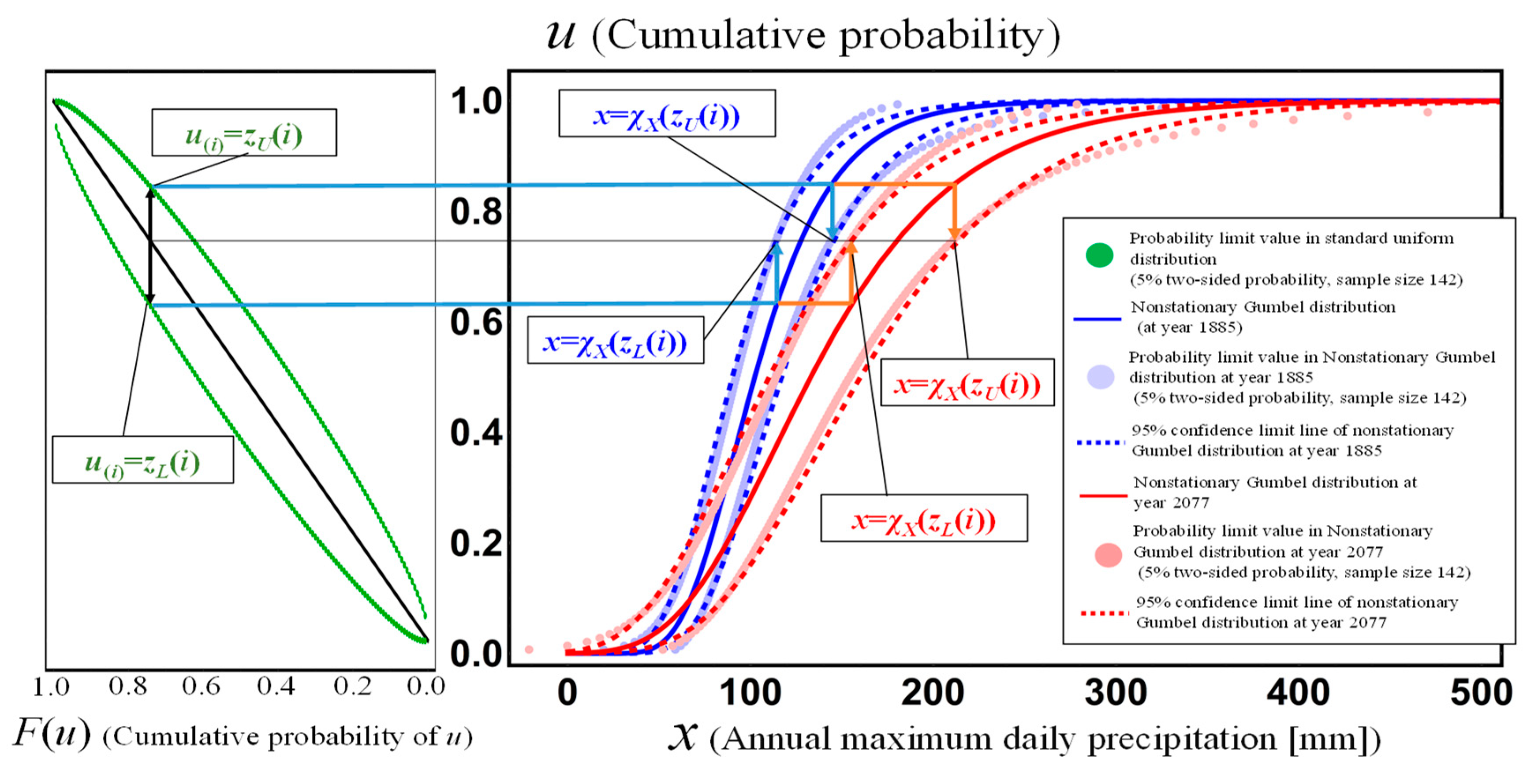
Figure 6 shows the construction process of the 95% confidence interval for the non-stationary extreme value distribution using probability limit method test. In the figure, the solid blue line and the dotted blue line are the non-stationary Gumbel distribution at 1885 and its 95% confidence limit line, and the solid red line and the dotted red line are the non-stationary Gumbel distribution at 2077 and its 95% confidence limit line. The green points represent the probability limit values in the standard uniform distribution, the blue points represent the probability limit values in the non-stationary Gumbel distribution at 1885, and the red points represent the probability limit values in the non-stationary Gumbel distribution at 2077. The probability limit values in the standard uniform distribution are determined according to the total number of observed data “n,” and they do not change with time. Also, while the non-stationary extreme value distribution changes with time, its cumulative probability follows the standard uniform distribution regardless of the type of probability distribution. Therefore, by substituting the probability limit value in the standard uniform distribution into the probability representing function of the non-stationary extreme value distribution at the target time, the probability limit value under that distribution can be calculated. This shows that the uncertainty of estimation is quantified according to the total number of observations accumulated to date, in the form of the width [z_L(i), z_U(i)] of the probability limit in the standard uniform distribution, and the range of possible annual maximum daily precipitation X_(i) [χ_X(z_L(i), t), χ_X(z_U(i), t)] is calculated at any time t from this width. Figure 6 shows the construction process of confidence interval of the Gumbel distribution at 1885 and 2077. As described above, the confidence limit line is the stationary extreme value distribution (Gumbel distribution in this study) fitted to the probability limit value at that time in the non-stationary extreme value distribution (in this study, the non-stationary Gumbel distribution). In this way, even in the non-stationary case, the special quality that the cumulative probability follows the standard uniform distribution can be used to construct a confidence interval based on probability limit method test.

6. Results and Discussion

As shown in the previous chapter, applying an analytical method for non-stationary hydrological frequency, the probability distribution of the extreme hydrological quantity can be estimated with time as an explanatory variable. This means that the same method can describe the time evolution of the probability distribution of extreme hydrological quantity, and that the probability distribution of extreme hydrological quantity in the past and future periods can be estimated.

In this chapter, the non-stationary hydrological frequency analysis, to which the confidence interval based on probability limit method test is introduced, is applied to past and future hydrological periods, and concrete examples are presented. Meanwhile, the probability of exceeding the upper confidence limit value is obtained by multiplying the “target return period” and the “one-sided probability of the confidence interval.” In other words, the risk that a heavy rainfall exceeding 100 (1 − p)% upper confidence limit value within the T-year probability can be expressed as (1/T) × p/2 [33,34,35], where p is the significance level and (1 − p) is the confidence coefficient (0 < p < 1). Note that, since the target data used the annual maximum value over 142 years from 1876 to 2017, the period before 2017 is defined as the past period, and the period after 2017 is defined as the future period in this paper.

6.1. Application of the Non-Stationary Hydrological Frequency Analysis, Introducing Confidence Interval to the Past Period

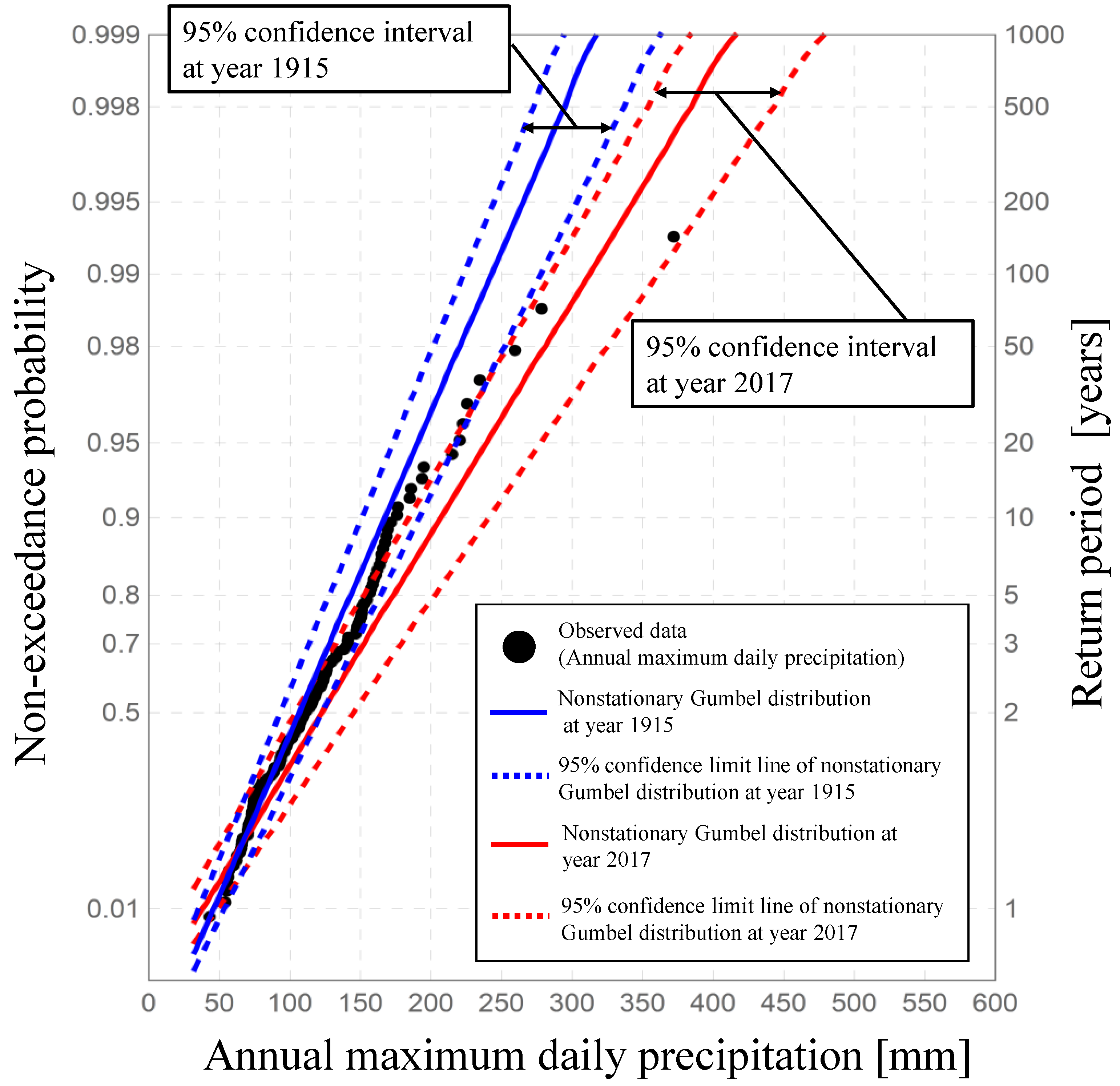
In this section, the non-stationary hydrological frequency analysis, to which the confidence interval was introduced, is applied to the past period to clarify temporal change of annual maximum daily precipitation. Figure 7 shows the observed data of the annual maximum daily precipitation over 142 years (from 1876 to 2017) at the ground observation station Tokyo, the non-stationary Gumbel distribution fitted to these 142 observed data, and 95% confidence interval of the non-stationary Gumbel distribution based on probability limit method test. Black dots denote observed data, blue solid line and blue dashed lines are the non-stationary Gumbel distribution and its 95% confidence limit lines, respectively, for 1915, and red solid line and red dashed line are the non-stationary Gumbel distribution and its 95% confidence limit lines, respectively, for 2017.

Figure 7 shows that the maximum daily precipitation derived from the non-stationary Gumbel distribution increases as the return period increases, and its confidence interval widens. It also can be seen in Figure 7 that the maximum value (371.9 mm) observed during the Typhoon Ida (1958), also known as the Kanogawa Typhoon, greatly deviates from the group of observation values below the upper second highest rank. Since this value greatly deviate from the non-stationary Gumbel distribution as of 1915 and 95% upper confidence limit line thereof, it becomes extremely difficult to evaluate this value using the confidence interval for 1915. Instead, this value was plotted in the vicinity of the 95% upper confidence limit lines as of 2017, and it becomes possible to perform probability evaluation of this value using the confidence interval. When the return period of this value is calculated using the 95% upper confidence limit lines for 2017, its return period becomes 123 years. Therefore, the risk of occurrence of a heavy rainfall exceeding this value, i.e., Typhoon Ida (in 1958)-class heavy rainfall, is 2.0 × 10⁻⁴ [=(1/123) × 2.5%, “target return period” × “one-sided probability of confidence interval” as per the framework of risk assessment [33,34,35] mentioned above. By introducing non-stationary hydrological frequency analysis to the confidence interval in order to evaluate uncertainty of T-year rainfall, we treat T-year rainfall as a random variable. Also, proposed confidence interval estimates the range of probability distribution of T-year rainfall. Therefore, an extremely heavy rainfall which deviates from a probability distribution fitted to past observed data can be interpreted as a realized value at right tail of the probability distribution of T-year rainfall. Moreover, above mentioned estimation method for occurrence risk of an extremely heavy rainfall is available, when considering an arbitrary return period of T-year. For example, considering the time development of probability distribution and confidence interval of 123-year rainfall, the amount of observed rainfall data (371.9 mm) in 1958, which is difficult to evaluate by the proposed 95% confidence interval in the time of 1915 becomes a realized value within the 95% confidence interval in 2017, i.e., a phenomenon that can be examined as a risk in flood control measures.

This result indicates that the occurrence risk of heavy rainfall similar to or more severe than extremely heavy rainfalls that have occurred in the past period is increasing. Moreover, the occurrence risk of such heavy rainfalls can be quantified by multiplying the target return period with the one-sided probability of the confidence interval, as described in the results of the non-stationary hydrological frequency analysis on the target data.

6.2. Application of the Non-Stationary Hydrological Frequency Analysis, Introducing Confidence Interval to the Future Period

In this section, the non-stationary hydrological frequency analysis method, to which the confidence interval was introduced, is applied to the future period to clarify expected changes in annual maximum daily precipitation. A period from 2017 until 2077 was defined as the target period to perform non-stationary hydrological frequency analysis. With non-stationary hydrological frequency analysis, the future distribution of the annual maximum daily precipitation in each year can be estimated over the 60-year period from 2017 to 2077.

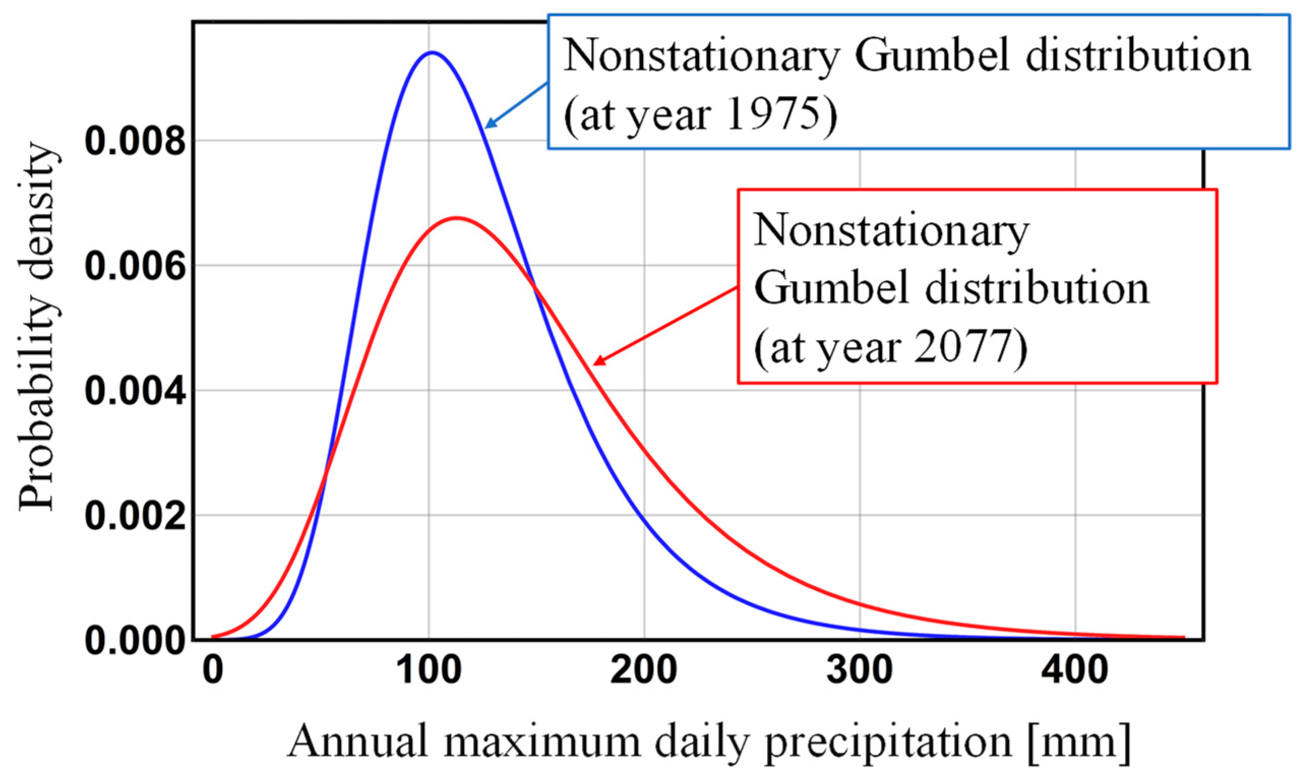
Figure 8 shows the non-stationary Gumbel distributions as of 1975, i.e., in the past period (blue solid line) and 2077, i.e., in the future (red solid line). It can be seen that the right tail of the Gumbel distribution in the future (red solid line) becomes wider than that in the past period (blue solid line) because of an increasing trend in annual maximum daily precipitation, and that the probability that the occurrence of heavy rainfall will increase.

Figure 9 shows observed data of annual maximum daily precipitation over 142 years (from 1876 to 2017) at the ground observation station Tokyo, the non-stationary Gumbel distribution fitted to these 142 observed data, and the 95% confidence interval of the non-stationary Gumbel distribution based on the probability limit method test. Black dots represent observed data, the blue solid and dashed lines are the non-stationary Gumbel distribution and its 95% confidence limit line, respectively, as of 1975, and red solid and dashed lines are the non-stationary Gumbel distribution and its 95% confidence limit line, respectively, as of 2077. There is an area in which the confidence intervals in the past and future periods overlap in Figure 9; therefore, it is understood that there was a possibility that the annual maximum daily precipitation in the future might also have occurred in the past period. In addition, the past maximum (371.1 mm) exceeds the 95% upper confidence limit value, whereas it is plotted near the average line (non-stationary Gumbel distribution, red solid line) in the future period. This indicates that Typhoon Ida-class heavy rainfalls can be expected to occur in the return period of 123-year in the future.

Although the risks presented by the product of “target return period” and “one-sided probability of upper confidence limit value” becomes the same values, probable rainfall corresponding to this risk changes depending on which point in time is considered. For example, the annual maximum daily precipitation corresponding to exceeding the probability of the 95% upper confidence limit value for the 100-year probability (=1/4000) was 323.9 mm in 1975, but will be 422.4 mm in 2077. By introducing the confidence interval into the non-stationary hydrological frequency analysis, the risk assessment for the occurrence of extremely heavy rainfall in the future becomes increasingly likely.

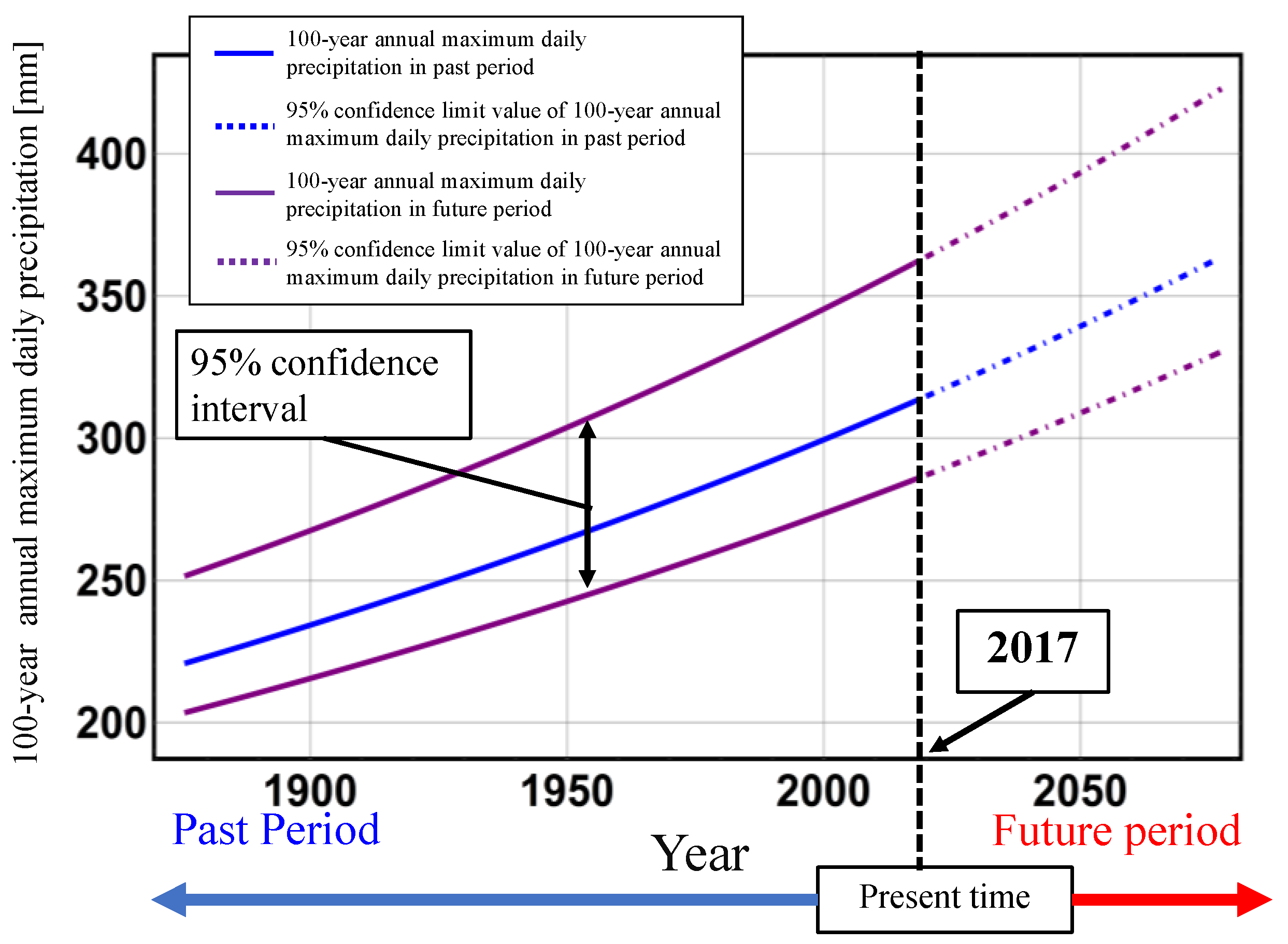
By applying the non-stationary hydrological frequency analysis method, temporal changes in the probability of heavy rainfall and the confidence limit value thereof can be estimated. Figure 10 shows 100-year annual maximum daily precipitation and a temporal change in the corresponding 95% confidence interval at the target location. The blue solid line shows the 100-year annual maximum daily precipitation in the past period, while the purple solid line is the 95% confidence limit line in the past period, the blue dashed-dotted line is 100-year annual maximum daily precipitation in the future, and the purple dashed-dotted line is the 95% confidence limit line in the future. This comparison shows that the above-mentioned quantities increase with time. By applying non-stationary hydrological frequency analysis, future changes in the probability of high hydrological quantities, and the confidence level of extreme values can be estimated.

In previous researches, confidence intervals are often expressed by using an assumption of normality to estimate statistics [37]. Our proposed confidence interval does not require such parametric assumptions as possible, and this confidence interval can be developed by incorporating the theory of probability limit method to non-stationary extreme value model shown by Coles [20], which can reflect the characteristic change of extreme time series with proceeding of time in this research.

In Japan, most design discharge in flood control measures is calculated by extracting hyetographs from past flood events, extrapolating the total amount of rainfall arising from those incidents up to the adopted probability scale, then converting this rainfall into a flow discharge using rainfall runoff modeling [41]. Shimizu et al. [42] demonstrated a method to convert confidence intervals regarding the hyetograph corresponding to a design scale into that of the calculated hydrograph using rainfall runoff modeling created by Yamada [43,44]. The rainfall runoff model created by Yamada gives prominence to parameters that consider the physical conditions of the outflow mechanism. By applying a non-stationary hydrological frequency analysis based on the confidence interval proposed in this study, the confidence interval of the peak flood discharge corresponding to the design scale under future climates can be constructed.

7. Conclusions

In recent years, increasing unsteadiness in the rainfall associated with climate change has become apparent; this is expected to continue in the future. Since previous design rainfalls have been set up based on an assumption of steadiness, the reliability of these design rainfalls may decrease because of unsteadiness in rainfall. Non-stationary hydrological frequency analysis is a method able to estimate rainfall corresponding to a design scale, while considering such changes in rainfall trend over time. The method enables a probable rainfall to be calculated as a function of time using a non-stationary extreme value distribution model with time as an explanatory variable. In this study, we developed a method to construct the confidence interval of the non-stationary extreme value distribution model by applying probability limit method test theory. In addition, it was shown that quantification of uncertainty in design rainfall because of a lack of observation information and an assessment of the occurrence risk of extremely heavy rainfall should consider changes in a trend in extreme rainfall series associated with climate change. This would be possible through the introduction of a confidence interval based on a probability limit method test incorporated into non-stationary hydrological frequency analysis.

The main results of this research are as follows.

(1)

It was shown that the confidence interval of the non-stationary extreme value distribution could be constructed using probability limit method test theory.

(2)

It was shown that the right tail of the non-stationary extreme value distribution fitted to a time series of observed data with increasing trend in rainfall widened with time, while its mode value increased. Also, it was shown that the confidence interval of the non-stationary extreme value distribution widened with the proceeding of time.

(3)

It was shown that, by introducing a confidence interval into the non-stationary hydrological frequency analysis, a risk assessment of the occurrence of extremely heavy rainfall considering the increasing trend of rainfall is possible.

(4)

It was shown that, by applying the non-stationary hydrological frequency analysis method, the confidence limit value of T-year rainfall in future time could be estimated. This result proposes quantification of occurrence risk for extremely heavy rainfall which could be treated as outliers in previous hydrological frequency analysis, and feasibility of introduction of occurrence risk these heavy rainfalls have into flood control management.

References

- Stedinger, J.R.; Vogel, R.M.; Foufoula-Georgiou, E. Frequency analysis of extreme events, Chapter 18. In Handbook of Hydrology; Maidment, D., Ed.; McGraw-Hill Professional: New York, NY, USA, 1993; pp. 18.1–18.66. [Google Scholar]
- Jain, S.; Lall, U. Floods in a changing climate, does the past represent the future? Water Resour. Res. 2001, 37, 3193–3205. [Google Scholar] [CrossRef]
- Wang, X.L.; Swail, V. Climate change signal and uncertainty in projections of ocean wave height. Clim. Dyn. 2006, 2, 109–126. [Google Scholar] [CrossRef]
- Wang, X.L.; Zwiers, F.W.; Swail, V. North Atlantic Ocean wave climate scenarios for the 21st century. J. Clim. 2004, 17, 2368–2383. [Google Scholar] [CrossRef]
- Kharin, V.V.; Zwiers, F.W. Estimating extremes in transient climate change simulations. J. Clim. 2005, 18, 1156–1173. [Google Scholar] [CrossRef]
- Climate Change Adaptation Research Group, National Institute for Land and Infrastructure Management, Ministry of Land, Infrastructure, Transport and Tourism, Japan. Technical Note of National Institute for Land and Infrastructure Management (Interim Report on Climate Change Adaptation Studies). No 749, Ⅱ-112-154. 2013. Available online: http://www.nilim.go.jp/lab/bcg/siryou/tnn/tnn0749pdf/ks0749.pdf (accessed on 12 September 2020).
- Milly, P.C.D.; Betancourt, J.; Falkenmark, M.; Hirsch, R.M.; Kundzewicz, Z.W.; Lettenmaier, D.P.; Stouffer, R.J. Stationarity is dead: Whither water management? Science 2008, 319, 573–574. [Google Scholar] [CrossRef] [PubMed]
- Sado, K.; Sugiyama, I.; Nakao, T. Renewal of probable hydrological amount using mean and variance jump—In case of annual maximum daily rainfall and number of days with continuous non-rainfall at 22 meteorological observatories in Hokkaido. Proc. Hydraul. Eng. Jpn. Soc. Civ. Eng. 2008, 52, 199–204. [Google Scholar] [CrossRef] [Green Version]
- Sogawa, N.; Suzuki, M. Long term nonstationarities of some fixed period precipitations over Japanese Islands in the 20th century and their influence upon the estimated values of the T-year return period precipitations. J. Jpn. Soc. Nat. Disaster Sci. 2008, 26, 355–365. [Google Scholar]
- Yamada, T.J.; Seang, C.N.; Hoshino, T. Influence of the long-term temperature trend on the number of new records for annual maximum daily precipitation in Japan. Atmosphere 2020, 11, 371. [Google Scholar] [CrossRef] [Green Version]
- Glick, N. Breaking records and breaking boards. Am. Math. Mon. 1978, 85, 2–26. [Google Scholar] [CrossRef]
- Galambos, J. Asymptotic Theory of Extreme Order Statistics; Wiley Series in Probability and Mathematical Statistics; John Wiley and Sons: Hoboken, NJ, USA, 1978. [Google Scholar]
- Kitano, K.; Takahashi, R.; Tanaka, S. Durability of an estimated 50 years-return-value over 50 years, discussed by introducing “diffractive effect” on the estimation error for flood frequency analysis. J. Jpn. Soc. Civ. Eng. (Hydraul. Eng.) 2012, 68, I_1375–I_1380. [Google Scholar]
- Kitano, K.; Morise, T.; Kioka, W.; Takahashi, R. Degree of experience in statistical analysis for extreme wave heights. Proc. Coast. Eng. Jpn. Soc. Civ. Eng. 2008, 55, 141–145. [Google Scholar] [CrossRef]
- Fisher, R.A.; Tippett, L.H.C. Limiting forms of the frequency distribution of the largest or smallest member of a sample. Proc. Camb. Philos. Soc. 1928, 24, 180–190. [Google Scholar] [CrossRef]
- Gumbel, E.J. Statistics of Extremes; Columbia University Press: New York, NY, USA, 1958. [Google Scholar]
- Gnedenko, B.V. Sur La Distribution Limite Du Terme Maximum D’Une Serie Aleatoire. Ann. Math. Second Ser. 1943, 44, 423–453. [Google Scholar] [CrossRef]
- Von Mises, R. La distribution de la plus grande de n values. Rev. Math. Union Interbalkanieque 1936, 1, 141–160. [Google Scholar]
- Jenkinson, A.F. The frequency distribution of the annual maximum (or minimum) values of meteorological elements. Quart. J. R. Meteorol. Soc. 1955, 81, 158–171. [Google Scholar] [CrossRef]
- Coles, S. An Introduction to Statistical Modeling of Extreme Values; Springer: London, UK, 2001. [Google Scholar]
- Khaliq, M.N.; Ourada, T.B.M.J.; Ondo, J.C.; Gachon, P.; Bobee, B. Frequency analysis of a sequence of dependent and/or non-stationary hydrometeorological observations: A review. J. Hydrol. 2006, 329, 534–552. [Google Scholar] [CrossRef]
- El Adlouni, S.; Ouarda, T.B.M.J.; Zhang, X.; Roy, R.; Bobee, B. Generalized maximum likelihood estimators for the nonstationary generalized extreme value model. Water Resour. Res. 2007, 43, W03410. [Google Scholar] [CrossRef]
- Towler, E.; Rajagopalan, B.; Gilleland, E.; Summers, R.S.; Yates, D.; Katz, R.W. Modeling hydrologic and water quality extremes in a changing climate. Water Resour. Res. 2010, 46, W11504. [Google Scholar] [CrossRef]
- Hayashi, H.; Tachikawa, Y.; Shiiba, M. Non-stationary hydrologic frequency analysis using time dependent parameters and its model selection. J. Jpn. Soc. Civ. Eng. (Hydraul. Eng.) 2015, 71, I_28–I_42. [Google Scholar]
- Akaike, H. A new look at the statistical model identification. IEEE Trans. Autom. Control 1974, 6, 716–723. [Google Scholar] [CrossRef]
- Takeuchi, K. Distribution of information statistics and criteria for adequacy of models. Mathemat. Sci. 1976, 153, 12–18. [Google Scholar]
- Neyman, J. Outline of a theory of statistical estimation based on the classical theory of probability. Philos. Trans. R. Soc. A 1937, 236, 333–380. [Google Scholar]
- Ministry of Land, Infrastructure, Transport, and Tourism (MLIT). Flood Control Technology Review Meeting Considering the Climate Change in Hokkaido Region. Available online: https://www.hkd.mlit.go.jp/ky/kn/kawa_kei/splaat000001offi.html (accessed on 31 August 2020).
- Yamada, T.J.; Hoshino, T.; Masuya, S.; Uemura, F.; Yoshida, T.; Omura, N.; Yamamoto, T.; Chiba, M.; Tomura, S.; Tokioka, S.; et al. The influence of climate change on flood risk in Hokkaido. Adv. River Eng. 2018, 24, 391–396. [Google Scholar]
- Yamada, T.J. Adaptation measures for extreme floods using huge ensemble of high-resolution climate model simulation in Japan. In Summary Report on the Eleventh Meeting of the Research Dialogue 2019, Proceedings of the UNFCCC Bonn Climate Change Conference, Bonn, Germany, 19 June 2019; pp. 28–30. Available online: https://unfccc.int/documents/197307 (accessed on 31 August 2020).
- Mizuta, R.; Murata, A.; Ishii, M. Over 5000 years of ensemble future climate simulations by 60-km global and 20-km regional atmospheric models. Bull. Am. Meteorol. Soc. 2016, 98, 1383–1393. [Google Scholar] [CrossRef]
- Fujita, M.; Mizuta, R.; Ishii, M.; Endo, H.; Sato, T.; Okada, Y.; Kawazoe, S.; Sugimoto, S.; Ishihara, K.; Watanabe, S. Precipitation changes in a climate with 2 K surface warming from large ensemble simulations using 60 km global and 20 km regional atmospheric models. Geophys. Res. Lett. 2018, 45, 435–442. [Google Scholar] [CrossRef] [Green Version]
- Shimizu, K.; Yamada, T.; Yamada, T.J. New hydrological frequency analysis introducing confidence interval of probability distribution models based on probability limit method test. J. Jpn. Soc. Civ. Eng. (Hydraul. Eng.) 2018, 74, I_331–I_336. [Google Scholar] [CrossRef]
- Shimizu, K.; Yamada, T.; Yamada, T.J. Projection for future change of confidence interval based on bayesian statistics using a large ensemble dataset. J. Jpn. Soc. Civ. Eng. (Hydraul. Eng.) 2019, 75, I_301–I_306. [Google Scholar]
- Shimizu, K.; Yamada, T.; Yamada, T.J. Uncertainty evaluation in hydrological frequency analysis based on confidence interval and prediction interval. Water 2020, 12, 2554. [Google Scholar] [CrossRef]
- Moriguti, S. Testing hypothesis on probability representing function—Kolmogorov–Smirnov test reconsidered. Jpn. J. Stat. Data Sci. 1995, 25, 233–244. [Google Scholar]
- Efron, B. The Jackknife, the Bootstrap, and other Resampling Plans; Society for Industrial and Applied Mathematics: Philadelphia, PA, USA, 1982. [Google Scholar]
- Moriguti, S. Probability Representing Function; Tokyo University Press: Tokyo, Japan, 1995. [Google Scholar]
- Kolmogorov, A. Sulla Determinazione Empiri-ca di una Legge di Distribuzione. Inst. Ital. Attuari Giorn. 1933, 4, 83–91. [Google Scholar]
- Smirnov, N. Ob uklonenijah empiriceskoi krivoi raspredelenija. Recl. Math. (Mathmaticeskii Sb.) 1939, 6, 3–26. [Google Scholar]
- Ministry of Land, Infrastructure, Transport and Tourism, Japan. Technical Criteria for River Works: Practical Guide for Planning. Available online: https://www.mlit.go.jp/river/shishin_guideline/gijutsu/gijutsukijunn/keikaku/index.html (accessed on 12 September 2020).
- Shimizu, K.; Yamada, T.; Yamada, T.J. Uncertainty Evaluation of Probable Flood Peak Discharge Using Confidence Interval Based on Probability Limit Method Test. J. Jpn. Soc. Civ. Eng. G (Environ. Res.) 2018, 74, I_293–I_302. [Google Scholar] [CrossRef]
- Yamada, T. Studies on nonlinear runoff in mountainous basins. Annu. J. Hydraul. Eng. 2003, 47, 259–264. [Google Scholar] [CrossRef]
- Yoshimi, K.; Yamada, T. Application of runoff analysis model considering vertical infiltraion to long- and short-term runoff. J. Jpn. Soc. Civ. Eng. (Hydraul. Eng.) 2018, 74, I_331–I_336. [Google Scholar]
Figure 1.
Time series showing observed data of the annual maximum daily precipitation over 142 years from 1876 to 2017 at the Meteorological Agency ground observation station Tokyo and the regression line fitted to this time series.
Figure 2.
Probability density function of the non-stationary Gumbel distribution applied to the observed data of the annual maximum daily precipitation over 142 years (from 1876 to 2017) at the Meteorological Agency ground observation station Tokyo. The axis of the depth direction represents the number of elapsed years.
Figure 3.
Time variation of the non-stationary Gumbel distribution applied to the observed data of annual maximum daily precipitation over 142 years (from 1876 to 2017) at the observation station Tokyo. The blue solid line represents the non-stationary Gumbel distribution in 1915, whereas the red solid line represents the non-stationary Gumbel distribution in 2017.
Figure 4.
Probability representing function of the Gumbel distribution χα(u) fitted to the sample of −log10(2αmin). In this study, 5000 αmin was sampled to secure the stability of the distribution of αmin.
Figure 5.
Probability limit lines with 5% two-sided probability in the standard uniform distribution. The symbol n represents the total number of observed data used to calculate the probability limit values.
Figure 6.
Construction process for the 95% confidence interval of the non-stationary extreme value distribution using probability limit method test. n is the total number of observed data. The blue solid and dashed lines are the non-stationary Gumbel distribution and its 95% confidence limit lines, respectively, for 1885. The red solid and dashed lines are the non-stationary Gumbel distribution and its 95% confidence limit lines, respectively, in 2077 (i.e., a future prediction). Green dots, blue dots, and red dots denote the probability limit values with a 5% two-sided probability in the standard uniform distribution, the non-stationary Gumbel distribution in 1885, and the non-stationary Gumbel distribution in 2077, respectively.
Figure 7.
Observed data of the annual maximum daily precipitation over 142 years (from 1876 to 2017. at the ground observation station Tokyo, together with the non-stationary Gumbel distribution fitted to these 142 observed data (blue solid line: non-stationary Gumbel distribution in 1915; red solid line, non-stationary Gumbel distribution in 2017), and the 95% confidence interval of both non-stationary Gumbel distributions based on probability limit method test. n is the total number of observed data. Note that the Hazen formula was used for the plotting position equation.
Figure 8.
Future changes in the non-stationary Gumbel distribution fitted to observed data of annual maximum daily precipitation over 142 years (from 1876 to 2017) at the ground observation station Tokyo. The blue solid line is the non-stationary Gumbel distribution in 1975 and the red solid line is the non-stationary Gumbel distribution in 2077.
Figure 9.
Observed data of annual maximum daily precipitation over 142 years (from 1876 to 2017) at the Meteorological Agency ground observation station Tokyo, with a non-stationary Gumbel distribution fitted to these values (blue solid line: non-stationary Gumbel distribution for 1975; red solid line, non-stationary Gumbel distribution for 2077). The 95% confidence intervals of both non-stationary Gumbel distributions are based on the probability limit method test. n is the total number of observed data. Note that the Hazen Equation was used for the plotting position equation.
Figure 10.
Temporal change of 100-year annual maximum daily precipitation and its 95% confidence interval.
© 2020 by the authors. Licensee MDPI, Basel, Switzerland. This article is an open access article distributed under the terms and conditions of the Creative Commons Attribution (CC BY) license (http://creativecommons.org/licenses/by/4.0/).
Share and Cite
MDPI and ACS Style
Shimizu, K.; Yamada, T.; Yamada, T.J. Introduction of Confidence Interval Based on Probability Limit Method Test into Non-Stationary Hydrological Frequency Analysis. Water 2020, 12, 2727. https://doi.org/10.3390/w12102727
AMA Style
Shimizu K, Yamada T, Yamada TJ. Introduction of Confidence Interval Based on Probability Limit Method Test into Non-Stationary Hydrological Frequency Analysis. Water. 2020; 12(10):2727. https://doi.org/10.3390/w12102727
Chicago/Turabian StyleShimizu, Keita, Tadashi Yamada, and Tomohito J. Yamada. 2020. "Introduction of Confidence Interval Based on Probability Limit Method Test into Non-Stationary Hydrological Frequency Analysis" Water 12, no. 10: 2727. https://doi.org/10.3390/w12102727
Note that from the first issue of 2016, this journal uses article numbers instead of page numbers. See further details here.