Variational Bayesian Neural Network for Ensemble Flood Forecasting

Abstract

Disastrous floods are destructive and likely to cause widespread economic losses. An understanding of flood forecasting and its potential forecast uncertainty is essential for water resource managers. Reliable forecasting may provide future streamflow information to assist in an assessment of the benefits of reservoirs and the risk of flood disasters. However, deterministic forecasting models are not able to provide forecast uncertainty information. To quantify the forecast uncertainty, a variational Bayesian neural network (VBNN) model for ensemble flood forecasting is proposed in this study. In VBNN, the posterior distribution is approximated by the variational distribution, which can avoid the heavy computational costs in the traditional Bayesian neural network. To transform the model parameters’ uncertainty into the model output uncertainty, a Monte Carlo sample is applied to give ensemble forecast results. The proposed method is verified by a flood forecasting case study on the upper Yangtze River. A point forecasting model neural network and two probabilistic forecasting models, including hidden Markov Model and Gaussian process regression, are also applied to compare with the proposed model. The experimental results show that the VBNN performs better than other comparable models in terms of both accuracy and reliability. Finally, the result of uncertainty estimation shows that the VBNN can effectively handle heteroscedastic flood streamflow data.

1. Introduction

Disastrous floods are destructive and likely to cause widespread economic losses [1]. Accurate and reliable flood forecasting may provide insightful information for water resource managers to assist in assessment of the flood risk and economic benefit [2,3]. Since 1980, many kinds of forecast models have been developed for flood forecasting, such as the moving average model [4,5], the support vector machine [6,7], and neural networks (NNs) [8,9,10]. Most of these models only give a point forecast value without any forecast uncertainty information [11]. However, there are always potential uncertainties in forecasting, and this uncertainty information also plays an important role in water resources management decision-making [12,13]. Therefore, it is important to develop appropriate ensemble or probability forecasting models to provide forecast uncertainty information for water resources managers.

Since 2000, a variety of approaches have been developed and applied to quantify the streamflow forecast uncertainty. A commonly used approach is to quantify the forecast uncertainty by estimating the lower and upper bound of the forecast interval (LUBE). The bounds usually represent the possible range of observed data with a certain probability of confidence (for example, 90%) [14]. The LUBE method was extended to NNs to estimate the output intervals of an NN model [15,16]. Another popular approach is to use Bayesian techniques to build Bayesian statistic models to quantify the forecast uncertainty. For example, the Bayesian joint probability forecast model is applied on monthly and seasonal streamflow forecasting [17,18,19]; Gaussian processes regression (GPR) with a Box–Cox transformation method is employed for monthly streamflow forecasting [20]; the Bayesian technique is used to derive the posterior probability distribution of hydrological model parameters, and the model is applied on daily streamflow forecasting [21]. Although the above references achieve the quantification of forecast uncertainty by different approaches, there are still some problems in these methods: (1) as for the LUBE method, an evolutionary optimization algorithm needs to be applied to optimize model parameters due to the coverage-width-based criterion cost function used in the LUBE method [15]. The deep neural network model has more hidden layers and larger dimension of neurons, so there will be millions of model parameters that need to be optimized. Therefore, LUBE is difficult to extend to a deep neural network due to the difficulty of parameter estimation [22]. (2) The Bayesian method uses prior distribution and likelihood function to calculate the posterior probability distribution of model parameters. This technology can effectively solve the problem of model overfitting and can use ensemble forecasting to quantify the uncertainty of model output [23,24]. However, the calculation process of the posterior distribution requires the computation of the Hessian matrix at each iteration, which will lead to challenging inference and at the same time lead to heavy calculation costs [25].

Variational inference is considered to be an alternative technique to solve computationally complex problems [26]. Its purpose is to find a model parameter optimization method that is convenient for training the NN to obtain the posterior distribution of model parameters. The main idea of variational inference is to obtain an approximate posterior distribution rather than the true posterior distribution of model parameters. The variational distribution is defined with variational parameters, and the objective is to obtain the optimal variational parameters that make the variational distribution close to the true posterior distribution. Inspired by the concept of variational inference, this paper applies variational inference to the BNN model and proposes a variational Bayesian neural network (VBNN) model for ensemble flood forecasting. The main contributions are summarized as follows:

(1)

The variational inference technique is used for the BNN model, and the variational lower bound of the VBNN is derived as the objective of the variational parameters. Monte Carlo method is applied in forecasting process, which converts model parameters’ uncertainty into model output uncertainty.

(2)

The VBNN is applied to a flood forecasting case study on the upstream of the Yangtze River. The performance of the VBNN is tested through several verification metrics. Experimental results show that the VBNN obtains better performance than other comparison models in terms of both accuracy and reliability.

(3)

Flood forecasting uncertainty estimation of the proposed ensemble forecasting model is shown. The experimental result shows that the VBNN can not only give accurate forecast results but also quantify the uncertainty of flood forecasting, which provides more useful information for water resources managers.

The remainder of this paper is organized as follows. In Section 2, the methodology of the VBNN is given in detail. Section 3 introduces the study area and data used in this paper. In Section 4, the experimental results of the VBNN and other comparison models are given. In Section 5, we give our conclusions.

2. Methodology

2.1. Bayesian Neural Network (BNN)

An NN consists of an input layer, hidden layers, and an output layer. In particularly, given the input data X = {x₁, …, x_N} and output data Y = {y₁, …, y_N} with N data points, the input and output data can be modeled with the parameters w as $\mathbf{Y}=\mathrm{NN}\left(\mathbf{X},w\right)$, where w can be trained by backpropagation. Then the model output value y* can be forecasted by giving a new input point x* through the network ${\mathbf{y}}^{*}=\mathrm{NN}\left({\mathbf{x}}^{*},w\right)$.

As for Bayesian neural networks, the values of the parameter w are initialized following a prior distribution p(w). Then the output and input training dataset X, Y is used to obtain the most optimal posterior distribution p(w|X, Y) of the BNN model parameters. According to the posterior distribution of parameters, the probability form of output can be derived by:

$$p\left({\mathbf{y}}^{*}|{\mathbf{x}}^{*},\mathbf{X},\mathbf{Y}\right)={\displaystyle \int p\left({\mathbf{y}}^{*}|{\mathbf{x}}^{*},w\right)}p\left(w|\mathbf{X},\mathbf{Y}\right)\mathrm{dw}$$

(1)

2.2. Variational Inference for BNN (VBNN)

According to the Bayes’ rule, the true posterior distribution of model parameters is calculated by the formulation p(w|X, Y) = p(w)p(X, Y|w)/p(X, Y), which involves the computation of intractable multidimensional integrals. Therefore, approximation techniques are needed to reduce calculation time. In this paper, variational inference is applied to handle the computationally complex problems. The objective of variational inference is to obtain the optimal variational parameters that make the variational distribution close to the true posterior distribution, which can be formulated as follows:

$$\mathrm{KL}\left(q_{\phi }\left(w\right)\Vert p\left(w|\mathbf{X},\mathbf{Y}\right)\right)=-{\displaystyle \int q_{\phi }\left(w\right)}\ln \left(\frac{p\left(w|\mathbf{X},\mathbf{Y}\right)}{q_{\phi }\left(w\right)}\right)\mathrm{dw}$$

(2)

where q_φ(w) is the variational distribution; φ represents the variational parameters, p(w|X, Y) is the true posterior distribution of model parameters; KL(a||b) represents the Kullback–Leibler (KL) divergence between distribution a and distribution b, the smaller the KL divergence, the closer the two distributions. However, it is still difficult to calculate Equation (2) directly. Therefore, the variational lower bound (VLB), an objective function with the same effect as KL divergence, is used in the VBNN model as the training loss function. The formulation of the VLB can be derived as follows:

$$\ln p\left(\mathbf{Y}|\mathbf{X}\right)=\ell \left(\phi \right)+\mathrm{KL}\left(q_{\phi }\left(w\right)\Vert p\left(w|\mathbf{X},\mathbf{Y}\right)\right)$$

(3)

$$\ell \left(\phi \right)={\displaystyle \int q_{\phi }\left(w\right)}\ln \left(\frac{p\left(\mathbf{Y},w|\mathbf{X}\right)}{q_{\phi }\left(w\right)}\right)\mathrm{dw}$$

(4)

where ln p(Y|X) is the conditional marginal log-likelihood, $\ell \left(\phi \right)$ is the variational lower bound. Since ln p(Y|X) is constant w.r.t. φ, minimizing the KL divergence is equal to maximizing VLB. The formulation of VLB can be written as follows:

$$\begin{array}{cc}\hfill \ell \left(\phi \right)& =L\left(\phi \right)-KL\left(q_{\phi }\left(w\right)\Vert p\left(w\right)\right)\hfill \\ & ={\displaystyle \int q_{\phi }\left(w\right)p\left(\mathbf{Y}|\mathbf{X},w\right)}\mathrm{dw}+{\displaystyle \int q_{\phi }\left(w\right)}\ln \left(\frac{p\left(w\right)}{q_{\phi }\left(w\right)}\right)\mathrm{dw}\hfill \end{array}$$

(5)

where L(φ) is the log-likelihood function, the larger the term, the better the model fits the data; the second term $KL\left(q_{\phi }\left(w\right)\Vert p\left(w\right)\right)$ can be regarded as a regular term, a small value means variational distribution q_φ(w) is close to the prior distribution p(w), which can effectively avoid the model overfitting phenomenon.

To train the VBNN without manually adjusting hyperparameters, this paper uses the variational dropout to adaptively optimize the variational parameters. In the variational dropout, the variational distribution q_φ(w_ij) is defined as a Gaussian distribution with mean θ_ij and variance σ_ij. The variational dropout can be expressed as follows:

$$q_{\phi }\left(w_{ij}\right)\sim \mathcal{N}\left({\theta }_{ij},{\sigma }_{ij}^2\right)$$

(6)

In VBNN, the variational parameters φ consist of θ_ij and σ_ij, φ = (θ, σ). The prior distribution p(w) is chosen as a standard Gaussian distribution $p\left(w_{ij}\right)\sim \mathcal{N}\left(0,1\right)$. Therefore, KL(q_φ(w)||p(w)) can be computed as follows:

$$\begin{array}{cc}\hfill -KL\left(q_{\phi }\left(w\right)\Vert p\left(w\right)\right)& ={\displaystyle \int q_{\phi }\left(w\right)}\ln \left(\frac{p\left(w\right)}{q_{\phi }\left(w\right)}\right)\mathrm{dw}\hfill \\ & ={\displaystyle \int q_{\phi }\left(w\right)}\left(\ln p\left(w\right)-\ln q_{\phi }\left(w\right)\right)\mathrm{dw}\hfill \\ & =\frac{1}{2}{\displaystyle \sum _{ij}\left(1+\ln {\sigma }_{ij}^2-{\theta }_{ij}^2-{\sigma }_{ij}^2\right)}\hfill \end{array}$$

(7)

After KL(q_φ(w)||p(w)) is derived, the log-likelihood term L(φ) in VLB is estimated as follows:

$$\begin{array}{cc}\hfill L\left(\phi \right)& ={\displaystyle \int q_{\phi }\left(w\right)p\left(\mathbf{Y}|\mathbf{X},w\right)}\mathrm{dw}\hfill \\ & \approx \frac{N}{M}{\displaystyle \sum _{m=1}^M\ln p\left({\mathbf{y}}_m|\mathrm{NN}\left({\mathbf{x}}_m,\widehat{w}\right)\right)},\widehat{w}\sim q_{\phi }\left(w\right)\hfill \end{array}$$

(8)

where M is the size of the mini-batch, $\widehat{w}$ is sample from the variational distribution. As for the regression NN model, the log-likelihood is equal to the negative square loss scaled by a constant $-{\Vert {\mathbf{y}}_m-{\mathrm{f}}_{\mathrm{Y}}^{\widehat{\omega }}({\mathbf{x}}_m)\Vert }^2+\mathrm{constant}$ [27]. Then, the VLB can be approximated:

$$\mathrm{VLB}\approx -\frac{N}{M}{\displaystyle \sum _{m=1}^M{\Vert {\mathbf{y}}_m-\mathrm{NN}\left({\mathbf{x}}_m,\widehat{w}\right)\Vert }^2}-\frac{1}{2}{\displaystyle \sum _{ij}\left(1+\log {\sigma }_{ij}^2-{\theta }_{ij}^2-{\sigma }_{ij}^2\right)}$$

(9)

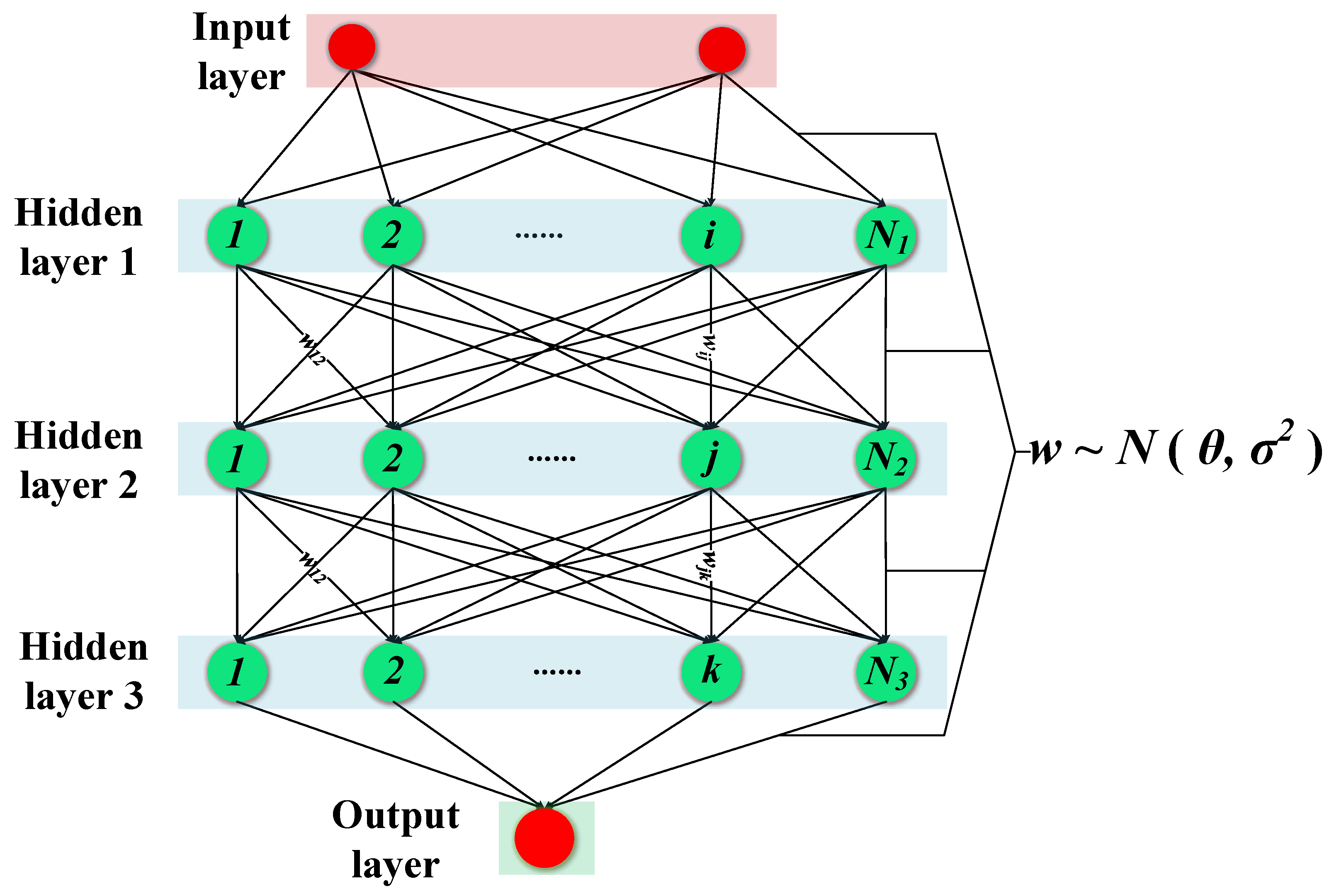
Finally, the VBNN model can be trained by maximizing the VLB. Figure 1 shows the network structure of the proposed VBNN. It can be seen from the figure that the difference between the VBNN and the traditional NN is that the weight parameter w between traditional NN nodes is a fixed value, while the weight parameter w of VBNN is a probability distribution q(w). Therefore, the traditional NN aims to optimize the weight parameter w during the training process, while the VBNN aims to optimize the parameters of the variational probability distribution φ = (θ, σ) during the training process.

2.3. Ensemble Forecasting

After training the VBNN model, we will obtain the optimal variational distribution q_φ(w), which is very close to the true posterior distribution p(w|X, Y) of model parameters. The variational distribution can reflect the uncertainty of model parameters. To transform the model parameters’ uncertainty into the model output uncertainty, the theoretical probability of y* can be given:

$$p\left({\mathbf{y}}^{*}|{\mathbf{x}}^{*}\right)={\displaystyle \int p\left({\mathbf{y}}^{*}|{\mathbf{x}}^{*},w\right)}\cdot q_{\phi }\left(w\right)\mathrm{dw}$$

(10)

The theoretical probability of y* is hard to calculate. Therefore, the Monte Carlo sampling method is used to obtain ensemble forecasting:

$$\begin{array}{c}\left[{\mathbf{y}}_1,{\mathbf{y}}_2,\dots ,{\mathbf{y}}_S\right]=NN\left({\mathbf{x}}^{*},\left[w_1,w_2,\dots ,w_S\right]\right)\\ \left[w_1,w_2,\dots ,w_S\right]\sim q_{\phi }\left(w\right)=\mathsf{\theta }+\mathsf{\sigma }ϵ\\ ϵ\sim \mathcal{N}\left(0,1\right)\end{array}$$

(11)

where S denotes the Monte Carlo sample number. In the sampling, S model parameters [w₁, w₂, …, w_s] are generated according to the variational distribution, then the ensemble forecasting result is obtained by forward passing through the network S times with different parameters sets.

2.4. Flowchart of VBNN

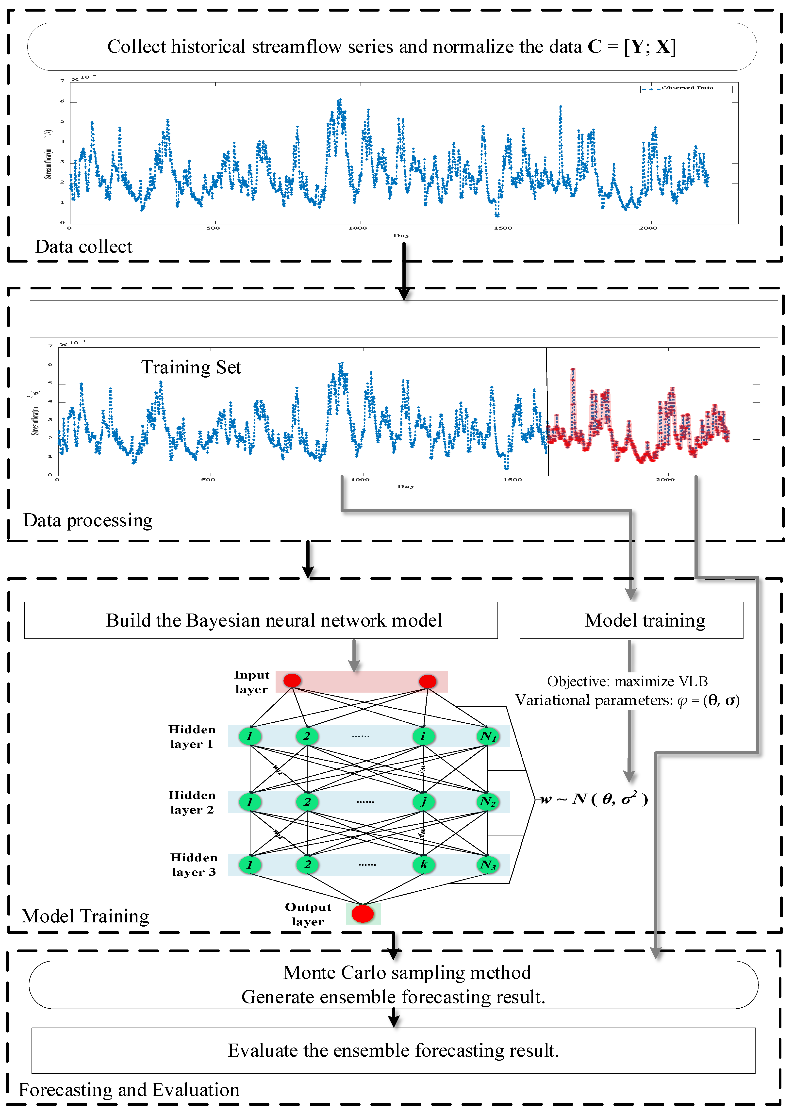
The flowchart of VBNN is shown in Figure 2. The complete steps are as follows:

Step 1: Collect historical streamflow series and normalize the data C = [Y; X].

Step 2: Divide the dataset into training set C_tranin = [Y_tranin; X_tranin] and test set C_teset = [Y_teset; X_teset].

Step 3: Determine the number of nodes in the input and output layers of the neural network model according to the dimensions of the input data and output data, set the number of hidden layers and the number of nodes in each layer.

Step 4: Train the VBNN using training set C_tranin = [Y_tranin; X_tranin]. The training objective is to maximize the VLB.

Step 5: According to the optimal variational parameters φ = (θ, σ), the Monte Carlo sampling method is used to generate an ensemble forecasting result.

Step 6: Evaluate the forecasting accuracy and reliability.

3. Study Area and Data

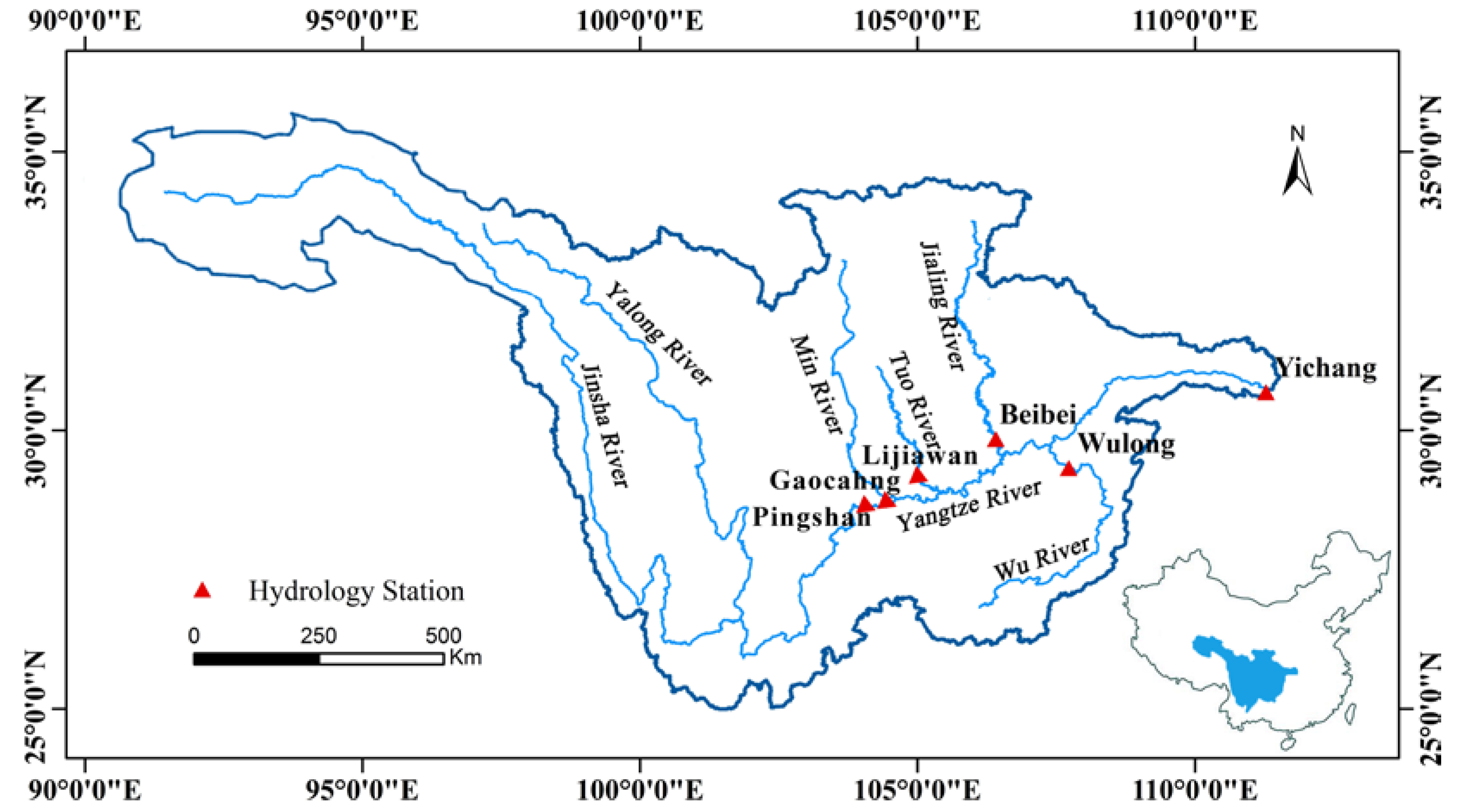
The upper Yangtze River basin, above Yichang, (Figure 3) was selected as our research area. The 6300 km long Yangtze River is the longest river in China and the third-longest in the world. The upper Yangtze River rises on the Qinghai–Tibet Plateau and flows through 6 provinces: Qinghai, Tibet, Sichuan, Yunnan, Chongqing, and Hubei. The basin is located between 90°33′ E to 112°25′ E and 24°30′ N to 35°45′ N, with a total area of 1.0 million square kilometers. The main tributaries are the Yalong River, Jingsha River, Min River, Tuo River, Jialing River, and Wu River. Throughout human history, this basin has experienced many large-scale floods, which have brought huge economic losses to the local country. Therefore, flood forecasting plays a vital role in the protection of human life and reduction of damage.

This study used hydrological data from six hydrological control stations in the upper Yangtze. From upstream to downstream, they are the Pingshan (ps), Gaochang (gc), Lijiawan (ljw), Beibei (bb), Wulong (wl), and Yichang stations (yc) (Figure 3). The streamflows of these six hydrological stations are taken as inputs, while the streamflow at Yichang station is the output. The data used covers a period of 55 years of daily mean streamflow during the flood season (June–September) from 1952 to 2006. The first 39 years (1952 to 1990) are used as the training dataset for parameter optimization, and the remaining 16 years (1991 to 2006) are used as test dataset for forecasting verification. The data after 2006 has not been used because the Three Gorges Dam started to operate after 2006, which will affect the distribution of streamflow. The inputs of the network are chosen from the antecedent streamflow. The output of the VBNN model is the streamflow of yc station Q_yc,t. Based on the correlation coefficient scores of the antecedent streamflow, the predictors are Q_yc,t−1, Q_yc,t−2, Q_ps,t−1, Q_gc,t−3, Q_bb,t−2, Q_wl,t−2, Q_ljw,t−3, where t represents the time step, the subscripts yc, ps, gc, bb, wl, and ljw represent the six hydrological stations above. The statistical information of the six hydrological stations is shown in the

Table 1. Statistical information of training dataset and test dataset.

Station	Training Set (m3/s)				Test Set (m3/s)
	Min	Max	Mean	std	Min	Max	Mean	std
Yichang	4120	69,500	25,223	10,012	4020	61,700	23,943	10,317
Pingshan	1380	28,600	8360	3925	1980	23,500	8809	4241
Gaochang	911	31,400	5319	2589	926	22,300	4731	2341
Lijiawan	24	14,500	882	1006	16	6720	647	832
Beibei	464	43,600	4443	4358	100	28,700	3283	3704
Wulong	288	19,900	2608	2322	368	20,400	2723	2547

. The minimum, maximum, mean, and standard deviation of the total dataset are abbreviated as min, max, mean, and std. From Table 1, we can see that the statistical information of Yichang, Pingshan, Gaochan, and Wulong stations is similar between training and test phases. However, the statistical information of Lijiawan and Beibei stations has some differences between training and test phases, which requires a more robust model.

4. Results and Verification

4.1. Model Development

In addition to the proposed VBNN, a deterministic prediction model NN and two probabilistic prediction models were developed for comparison, including Gaussian process regression (GPR) and hidden Markov model (HMM) [28].

(1)

VBNN: In this paper, the VBNN consisted of 1 input layer, 3 hidden layers (the neural network node of each hidden layer was set as 40), and 1 output layer. A stochastic optimization method, Adam [29], was used to train the VBNN. In this study, the learning rate of Adam was set as 0.001 and the epoch was 10,000.

(2)

NN: In order to compare with the VBNN model, an NN was also developed for this flood forecasting case. The network structure of NN was the same as that of the VBNN. The optimization method, learning rate, and epoch were also the same as those of the VBNN.

(3)

GPR: An NN was devolved mainly to compare the forecast accuracy of VBNN. The GPR was devolved for forecast reliability comparison. GPR is a popular machine learning method that can give probabilistic predictions.

(4)

HMM: HMM is also a powerful probabilistic forecasting model. In HMM, the expectation-maximization algorithm was firstly executed, and then Gaussian mixture regression method was used to give the conditional probability density function of the forecasted flood.

4.2. Verification Metrics

To verify the forecast accuracy of the flood forecasting model, root mean square error (RMSE) is used. The formulation is as follows:

$$RMSE=\sqrt{\frac{1}{T}{\displaystyle \sum _{t=1}^T{\left(y_t^p-y_t^{obs}\right)}^2}}$$

(12)

where $y_t^p$ is predicted streamflow at time t, $y_t^{obs}$ is observed streamflow at time t, T is the total number of forecasts. A smaller value of RMSE means better accuracy of the forecast.

The Nash–Sutcliffe efficiency coefficient (NSE) is a common evaluation index used to assess the predictive power of hydrological models. It is defined as:

$$\mathrm{NSE}=1-\frac{{\displaystyle {\sum }_{t=1}^T{\left(y_t^p-y_t^{obs}\right)}^2}}{{\displaystyle {\sum }_{t=1}^T{\left(y_t^{obs}-{\overline{y}}^{obs}\right)}^2}}$$

(13)

where ${\overline{y}}^{obs}$ is the mean observed streamflow. The NSE ranges from −∞ to 1. An efficiency of 1 (NSE = 1) corresponds to a perfect match of the predicted streamflow to the observed data. An efficiency of 0 (NSE = 0) indicates that the predictions are as accurate as the mean of the observed data.

In addition to verifying the accuracy of the forecasting model by RMSE, the continuous ranked probability score (CRPS)was also used in this study. This metric not only involves the forecast accuracy but also considers the forecast range of ensemble forecasting or probabilistic forecasting [30]. It can be formulated as follows:

$$CRPS=\frac{1}{T}{\displaystyle \sum _{t=1}^T{\displaystyle {\int }_{-\infty }^{+\infty }{\left[F_t\left(x\right)-H\left(x-y_t^{obs}\right)\right]}^{2}dx}}$$

(14)

where T is the time length of the forecasting task, $y_t^{obs}$ is the t-th observed value, F_t(x) is the cumulative distribution function for the t-th forecast, $H\left(x-y_t^{obs}\right)$ is the Heaviside function, and the definitions of F_t(x) and $H\left(x-y_t^{obs}\right)$ are as follows:

$$F_t\left(x\right)={\displaystyle {\int }_{-\infty }^{x}p\left(y_t\right)d{y}_t}$$

(15)

$$H\left(x-y_t^{obs}\right)=\{\begin{array}{ll}0& \mathrm{for}(x-y_t^{obs})<0\\ 1& \mathrm{for}(x-y_t^{obs})\ge 0\end{array}$$

(16)

where p(y_t) is the predictive probability of y_t. The smaller the CRPS value, the more reasonable the forecast distribution given by the model. The minimum value of CRPS is 0, which only appears in the case of a perfect prediction.

4.3. Results

4.3.1. Forecasting Skill Verification

The RMSE, NSE, and CRPS values of the four models during the test time (1991–2008 year) are given in

Table 2. The root mean square error (RMSE), Nash–Sutcliffe efficiency coefficient (NSE), and continuous ranked probability score (CRPS) of VBNN, neural network (NN), Gaussian process regression (GPR), and hidden Markov model (HMM) during the test time.

Year	RMSE (m3/s)				NSE				CRPS (m3/s)
	VBNN	NN	GPR	HMM	VBNN	NN	GPR	HMM	VBNN	GPR	HMM
1991	1809	1998	1807	1821	0.9588	0.9497	0.9589	0.9582	882	907	971
1992	1076	1442	1099	1102	0.9815	0.9668	0.9807	0.9806	583	615	684
1993	1493	1501	1794	1580	0.9834	0.9832	0.976	0.9814	810	1047	909
1994	1309	1409	1404	1310	0.9352	0.9249	0.9255	0.9351	519	666	572
1995	1464	1634	1416	1412	0.9358	0.9201	0.94	0.9404	771	754	760
1996	1715	1628	1640	1549	0.9588	0.9629	0.9623	0.9664	784	767	754
1997	1487	1571	1635	1524	0.9737	0.9707	0.9682	0.9724	666	852	780
1998	2887	2615	2759	2625	0.9669	0.9729	0.9698	0.9727	1339	1380	1305
1999	1788	1747	1735	1668	0.97	0.9714	0.9718	0.9739	886	868	877
2000	1889	1899	1859	1788	0.9547	0.9542	0.9561	0.9594	886	880	855
2001	1118	1587	1219	1262	0.978	0.9557	0.9739	0.972	628	684	708
2002	1262	1396	1251	1173	0.9824	0.9785	0.9827	0.9848	586	613	578
2003	2343	2463	2717	2476	0.9437	0.9378	0.8731	0.8831	1259	1836	1807
2004	1900	2010	1927	1973	0.9333	0.9308	0.9364	0.9382	952	954	988
2005	1690	1845	1754	1747	0.9692	0.9657	0.969	0.9712	807	783	835
2006	1050	1137	1630	1446	0.9481	0.9392	0.8248	0.9015	585	1312	1001
mean	1643	1743	1728	1654	0.9608	0.9553	0.9481	0.9557	815	913	889

Note: Bold values indicate the best metrics.

, the best metrics are bolded. The average RMSE of the VBNN was 1643, which is the best among these four models. The NN models obtained the worst RMSE value among the four comparison models, which may have been caused by overfitting. Compared to the NN model, the VBNN had a 5.74% lower average RMSE value over all prediction tasks, and GPR and HMM obtained a 0.86% and 5.11% lower average RMSE value on average over all prediction tasks. The proposed VBNN model outperformed other models in the most forecasting tasks in terms of RMSE and NSE, which demonstrates the forecasting accuracy of the VBNN. The RMSE and NSE can only evaluate the accuracy of a deterministic forecast and are not suitable for giving a comprehensive evaluation of ensemble forecasts or probability forecasts. CRPS is able to provide a comprehensive evaluation of the forecast accuracy and reliability. From Table 2, the VBNN still outperforms other probabilistic forecasting models in the case of CRPS values in the most forecasting tasks, which demonstrates its ability both on accuracy and reliability.

It can be seen from the experimental results that, although the VBNN model was better than other models in most years, there were still situations where other models were better than the VBNN in some years. This phenomenon shows that no model can be better than all other models at all prediction points. It also proves that there is uncertainty in forecasting models. The pros and cons of a model cannot be measured solely from the forecast accuracy of a certain year, and the reliability of the model forecast needs to be verified. Next, a more detailed verification of forecast reliability is given by probability integral transform (PIT) histogram and reliability diagrams.

4.3.2. Reliability of Forecasting

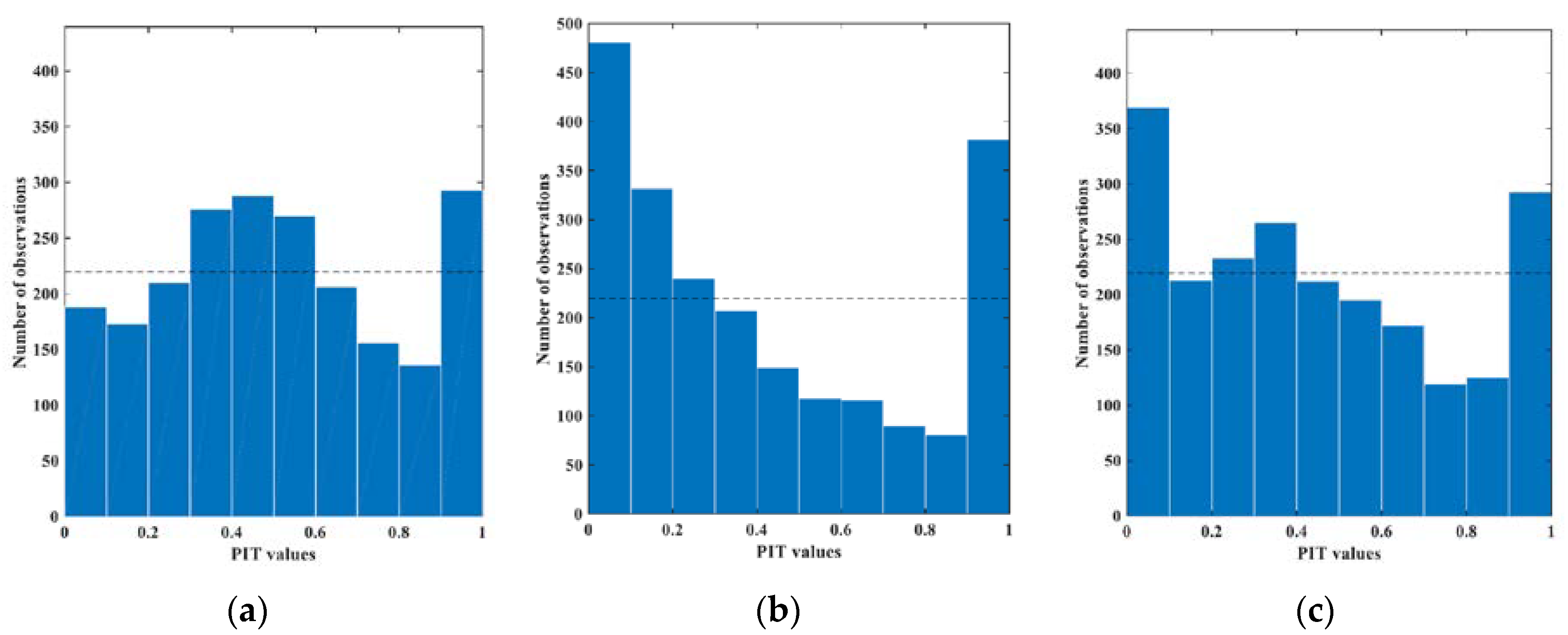
Unlike the deterministic forecasting model, ensemble forecasting model and probabilistic forecasting model not only give forecast points but also provide the forecast intervals. If the forecast interval is too wide, it means that the model has overestimated the uncertainty of the forecast. If the forecast interval is too narrow, it means the model has underestimated the uncertainty of the forecast. Therefore, if the forecast interval is too wide or too narrow, the reliability of the model will be very low. In this paper, the probability integral transform (PIT) value was used to evaluate the reliability of forecasting. The PIT values can be calculated from the frequency of ensemble forecasts that are lower than the observed streamflow. The PIT value ranges from 0 to 1. If most of the PIT values are near 0 or 1, it proves that the forecast interval is too narrow. If most of the PIT values are near 0.5, it proves that the forecast interval is too wide. According to the literature [31], if the PIT value follows a uniform distribution, the prediction is considered reliable. The reliability of forecast intervals is shown using PIT histograms in Figure 4. The horizontal axis of the PIT histogram means different bins of PIT values, while the vertical axis is the number of observations existing in every bin, and the black horizontal dashed line means the theoretical uniform frequency. As shown in Figure 4, the PIT histograms with VBNN, GPR, and HMM were plotted, and the frequency of every bin was, in general, near the theoretical uniform frequency for VBNN and HMM. However, most of the PIT values of GPR were distributed in [0, 0.1] and [0.9, 1], which means the spread of the forecast was too narrow. The figures show that the distribution of PIT values obtained by VBNN is quite uniform without too many excessively prediction values, which indicates that the ensemble forecasting results are reliable. Therefore, we believe that the ensemble forecast of proposed VBNN is generally unbiased and with appropriate spread.

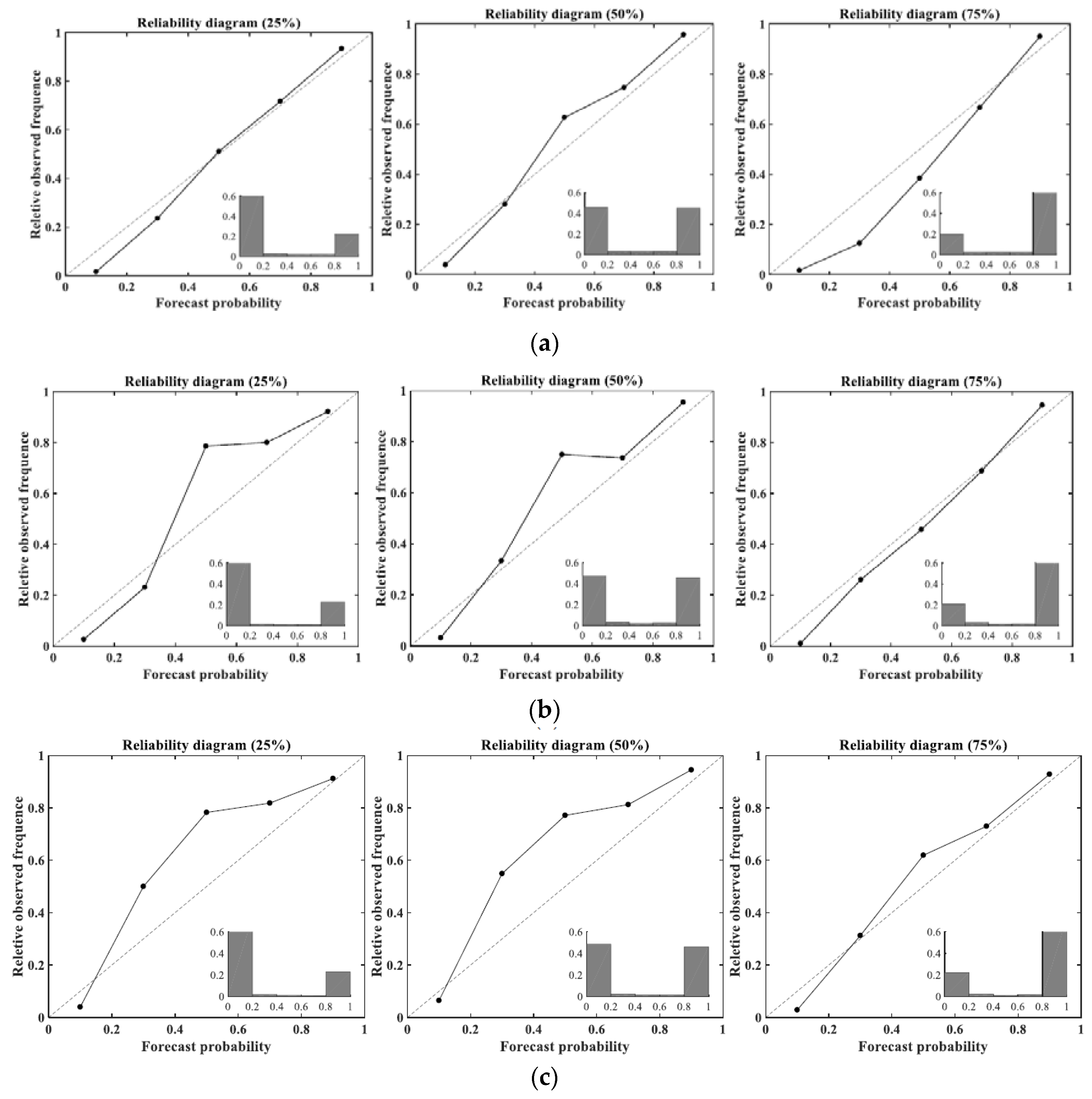
In addition to the PIT histograms, the reliability diagrams for an event smaller than the 25%, 50%, or 75% quantile of historical flows obtained by the three models are shown in Figure 5. The forecast probability is divided into 5 areas from 0 to 1 at intervals of 0.2. The reliability diagrams show that the forecast reliability and observed relative frequency matched well with the diagonal line. As shown in Figure 5, the forecast probabilities and observed frequency from the VBNN model were very close to the 1:1 line in case of all 25%, 50%, and 75% events. However, the GMR and HMM obtained a 1:1 line in the case of a 75% event but failed in the case of 25% and 50% events. Therefore, we consider that the ensemble forecasts of VBNN are reasonably consistent with the probabilities of all 25%, 50%, and 75% events occurring. The forecasts of GPR and HMM may be reliable with the probabilities of 75% events but less reliable in the case of 25% and 50% events.

4.3.3. Uncertainty Estimation

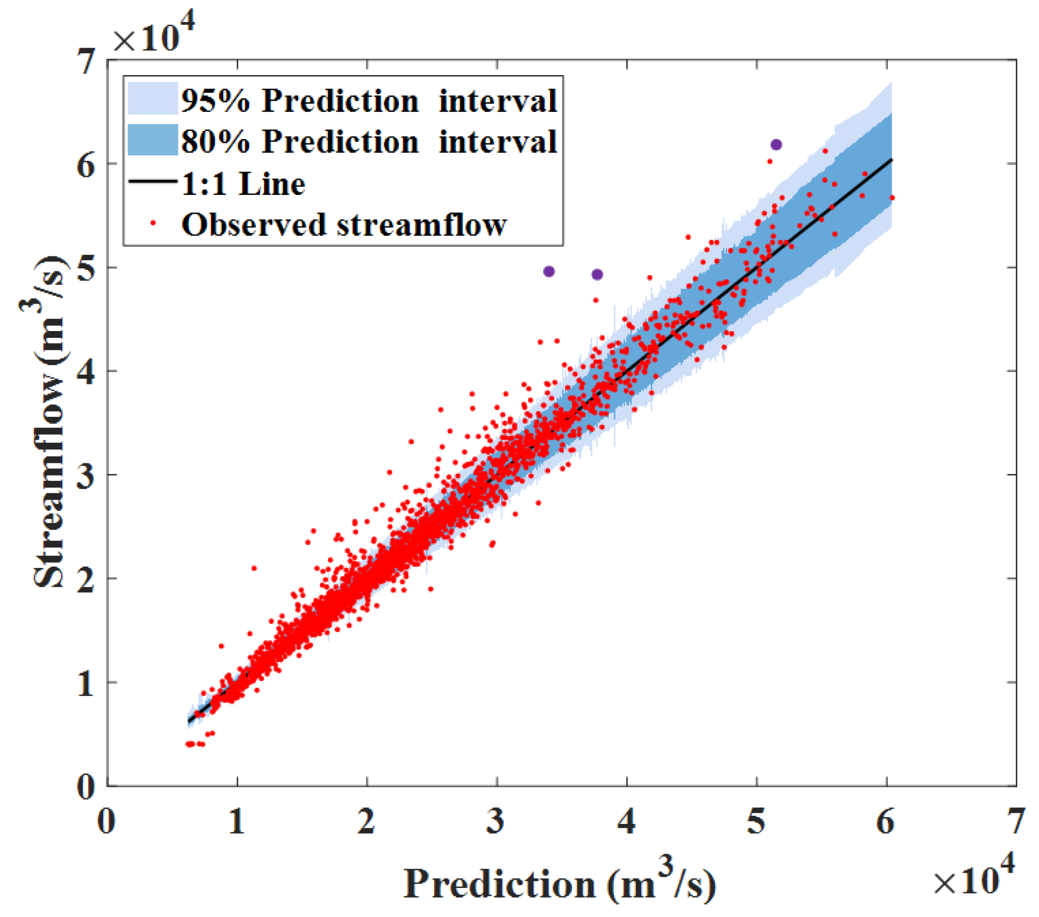
The prediction accuracy and reliability of the four comparison models are shown above. Next, we focus on the analysis of the forecast uncertainty of the proposed VBNN model. Figure 6 shows the uncertainty estimation of VBNN’s forecast results during whole test time. In the figure, the horizontal axis is the mean value of the ensemble forecast, the vertical axis is the relative observed streamflow, the light blue patch and blue patch are 95% and 80% credible intervals of model forecasts. It can be seen from Figure 6 that VBNN obtains a linear relationship between the forecast mean value and true observed streamflow value. This phenomenon shows that the forecast mean value is highly consistent with the true flood streamflow and has a high forecast accuracy. The uncertainty of the ensemble forecast can be quantified by 80% and 95% credible intervals, as seen from Figure 6, the uncertainty of the forecast is expanded as the forecast value increases. In other words, the variance of ensemble forecast was large when it predicted a big streamflow and the variance became smaller when the forecast streamflow was also small. In the figure, three purple nodes are regarded as outliers, and these three outliers appeared on 2 July 1998, 16 August 1998, and 2 July 2020, respectively. We found that these three points were sudden change points (the previous runoff was not large, but it suddenly increased at this moment). By analyzing the corresponding predictors at the three moments, no sudden changes of the predictors were found. This phenomenon proves that outliers are not caused by the model, but the selected predictors cannot effectively capture this sudden streamflow change. Therefore, more work on predictor selection is needed in the future to enhance the forecast accuracy of the model.

Due to the whole evaluation period being too long, we only plotted hydrological maps for 1998 and 2004, in which the entire Yangtze River Basin suffered severe floods. Figure 7 shows the forecast uncertainty for the 1998 and 2004 flood season in chronological order. Similar to Figure 6, Figure 7 shows that when the model predicted a larger flood, it was often accompanied by larger forecast uncertainty. This result demonstrates that the VBNN model can effectively handle heteroscedastic flood streamflow data. Therefore, the proposed VBNN can not only give accurate forecast results but also quantify the uncertainty of flood forecasting, which provides more useful information for water resources managers.

5. Conclusions

This study proposes a VBNN model for ensemble flood forecasting. To avoid heavy computational costs in the traditional BNN, the VBNN combines the variational inference with BNN, and uses the variational distribution to approximate the true posterior distribution of model parameters. To find the closest variational distribution to the true posterior distribution, the variational lower bound was derived as the model cost function. Monte Carlo sampling method was applied to give the ensemble forecasting results in order to transform the model uncertainty into the model forecasting uncertainty. The proposed method was verified by a flood forecasting case study on the upper Yangtze River. A point forecasting model neural network and two probabilistic forecasting models including HHM and GPR were also applied to compare with the proposed model. We summarize the conclusions as follows: (1) The VBNN obtained more accurate forecast results than the other three comparison models. (2) The forecast reliability of the VBNN was better than that of the other two probability forecast models GPR and HMM. (3) The VBNN could quantify reasonable forecast uncertainty for flood forecasting and could effectively handle heteroscedastic flood streamflow data.

Several possible extensions may be considered to the model proposed in this study. In particular, the predictor selection procedure, which would improve the forecast accuracy. Dam construction and operation influence the streamflow, the general method is to use the data after the dam is built to train the model, which greatly reduces the number of training sets. A more general streamflow forecasting model needs to be established, which can provide accurate forecasts in both the natural period and the period after the dam is in operation.

References

- Cutter, S.L.; Ismail-Zadeh, A.; Alcántara-Ayala, I.; Altan, O.; Baker, D.N.; Briceño, S.; Gupta, H.; Holloway, A.; Johnston, D.; McBean, G.A.; et al. Global risks: Pool knowledge to stem losses from disasters. Nature 2015, 522, 277–279. [Google Scholar] [CrossRef] [PubMed]
- Liu, Y.; Qin, H.; Mo, L.; Wang, Y.; Chen, D.; Pang, S.; Yin, X. Hierarchical flood operation rules optimization using multi-objective cultured evolutionary algorithm based on decomposition. Water Resour. Manag. 2018. [Google Scholar] [CrossRef]
- Liu, Y.; Qin, H.; Zhang, Z.; Yao, L.; Wang, Y.; Li, J.; Liu, G.; Zhou, J. Deriving reservoir operation rule based on bayesian deep learning method considering multiple uncertainties. J. Hydrol. 2019, 579, 124207. [Google Scholar] [CrossRef]
- Haltiner, J.P.; Salas, J.D. Short-term forecasting of snowmelt runoff using ARMAX models. J. Am. Water Resour. Assoc. 1988, 24, 1083–1089. [Google Scholar] [CrossRef]
- Salas, J.D.; Iii, G.Q.T.; Bartolini, P. Approaches to multivariate modeling of water resources time series 1. J. Am. Water Resour. Assoc. 1985, 21, 683–708. [Google Scholar] [CrossRef]
- Dibike, Y.B.; Velickov, S.; Solomatine, D.; Abbott, M.B. Model induction with support vector machines: Introduction and applications. J. Comput. Civ. Eng. 2001, 15, 208–216. [Google Scholar] [CrossRef]
- Wu, C.L.; Chau, K.W.; Li, Y.S. Predicting monthly streamflow using data-driven models coupled with data-preprocessing techniques. Water Resour. Res. 2009, 45, 2263–2289. [Google Scholar] [CrossRef] [Green Version]
- Mutlu, E.; Chaubey, I.; Hexmoor, H.; Bajwa, S.G. Comparison of artificial neural network models for hydrologic predictions at multiple gauging stations in an agricultural watershed. Hydrol. Process. 2008, 22, 5097–5106. [Google Scholar] [CrossRef]
- Castellano-Méndez, M.A.; González-Manteiga, W.; Febrero-Bande, M.; Prada-Sánchez, M.J.; Lozano-Calderón, R. Modelling of the monthly and daily behaviour of the runoff of the Xallas river using Box-Jenkins and neural networks methods. J. Hydrol. 2004, 296, 38–58. [Google Scholar] [CrossRef]
- Chiang, Y.; Chang, L.; Chang, F. Comparison of static-feedforward and dynamic-feedback neural networks for rainfall-runoff modeling. J. Hydrol. 2004, 290, 297–311. [Google Scholar] [CrossRef]
- Nash, J.E.; Sutcliffe, J.V. River flow forecasting through conceptual models part I—A discussion of principles. J. Hydrol. 1970, 10, 282–290. [Google Scholar] [CrossRef]
- Cloke, H.L.; Pappenberger, F. Ensemble flood forecasting: A review. J. Hydrol. 2009, 375, 613–626. [Google Scholar] [CrossRef]
- Shrestha, D.L.; Robertson, D.E.; Bennett, J.C.; Wang, Q.J. Improving precipitation forecasts by generating ensembles through postprocessing. Mon. Water Weather Rev. 2015, 143, 3642–3663. [Google Scholar] [CrossRef]
- De Gooijer, J.G.; Hyndman, R.J. 25 years of time series forecasting. Int. J. Forecast. 2006, 22, 443–473. [Google Scholar] [CrossRef] [Green Version]
- Khosravi, A.; Nahavandi, S.; Creighton, D.; Atiya, A.F. Lower upper bound estimation method for construction of neural network-based prediction intervals. IEEE Trans. Neural Netw. 2011, 22, 337–346. [Google Scholar] [CrossRef]
- Ye, L.; Zhou, J.; Gupta, H.V.; Zhang, H.; Zeng, X.; Chen, L. Efficient estimation of flood forecast prediction intervals via single- and multi-objective versions of the lube method. Hydrol. Process. 2016, 30, 2703–2716. [Google Scholar] [CrossRef]
- Wang, Q.J.; Robertson, D.E.; Chiew, F.H.S. A Bayesian joint probability modeling approach for seasonal forecasting of streamflows at multiple sites. Water Resour. Res. 2009, 45, 641–648. [Google Scholar] [CrossRef]
- Wang, Q.J.; Robertson, D.E. Multisite probabilistic forecasting of seasonal flows for streams with zero value occurrences. Water Resour. Res. 2011, 47, 155–170. [Google Scholar] [CrossRef]
- Zhao, T.; Schepen, A.; Wang, Q.J. Ensemble forecasting of sub-seasonal to seasonal streamflow by a Bayesian joint probability modelling approach. J. Hydrol. 2016, 541, 839–849. [Google Scholar] [CrossRef]
- Sun, A.Y.; Wang, D.; Xu, X. Monthly streamflow forecasting using Gaussian Process Regression. J. Hydrol. 2014, 511, 72–81. [Google Scholar] [CrossRef]
- Ye, L.; Zhou, J.; Zeng, X.; Guo, J.; Zhang, X. Multi-objective optimization for construction of prediction interval of hydrological models based on ensemble simulations. J. Hydrol. 2014, 519, 925–933. [Google Scholar] [CrossRef]
- Liu, Y.; Qin, H.; Zhang, Z.; Pei, S.; Jiang, Z.; Feng, Z.; Zhou, J. Probabilistic spatiotemporal wind speed forecasting based on a variational Bayesian deep learning model. Appl. Energy 2020. [Google Scholar] [CrossRef]
- Mackay, D.J.C. A practical bayesian framework for backpropagation networks. Neural Comput. 1992, 4, 448–472. [Google Scholar] [CrossRef]
- Neal, R.M. Bayesian Learning for Neural Networks. Ph.D. Thesis, University of Toronto, Toronto, ON, Canada, 1995. [Google Scholar]
- Taormina, R.; Chau, K. ANN-based interval forecasting of streamflow discharges using the LUBE method and MOFIPS. Eng. Appl. Artif. Intell. 2015, 45, 429–440. [Google Scholar] [CrossRef]
- Bishop, C.M. Pattern Recognition and Machine Learning (Information Science and Statistics); Springer: New York, NY, USA, 2006. [Google Scholar]
- Tishby; Levin; Solla. Consistent inference of probabilities in layered networks: Predictions and generalizations. In Proceedings of the International 1989 Joint Conference on Neural Networks, Washington, DC, USA, 6 August 2002; pp. 403–409. [Google Scholar]
- Liu, Y.; Ye, L.; Qin, H.; Hong, X.; Ye, J.; Yin, X. Monthly streamflow forecasting based on hidden Markov model and Gaussian Mixture Regression. J. Hydrol. 2018, 561, 146–159. [Google Scholar] [CrossRef]
- Kingma, D.P.; Ba, J. Adam: A method for stochastic optimization. In Proceedings of the 3nd International Conference on Learning Representations 2015, San Diego, CA, USA, 7–9 May 2015. [Google Scholar]
- Hersbach, H. Decomposition of the continuous ranked probability score for ensemble prediction systems. Weather Forecast. 2000, 15, 559–570. [Google Scholar] [CrossRef]
- Laio, F.; Tamea, S. Verification tools for probabilistic forecasts of continuous hydrological variables. Hydrol. Earth Syst. Sci. 2007, 11, 1267–1277. [Google Scholar] [CrossRef] [Green Version]
Figure 1.
Network structure of variational Bayesian neural network (VBNN).
Figure 2.
The flowchart of VBNN.
Figure 3.
Location of the stations on the upstream of Yangtze River.
Figure 4.
Probability integral transform (PIT) histograms: (a) VBNN, (b) GPR, (c) HMM (black horizontal dashed line: the theoretical uniform frequency).
Figure 5.
Reliability diagrams for an event smaller than the 25%, 50%, or 75% of historical flows obtained by: (a) VBNN, (b) GPR, (c) HMM.
Figure 6.
Uncertainty estimation of forecasts during whole test time (red dot, scatter point of predictions and observed streamflows; black line, 1:1 line; blue band, 80% credible interval; light blue band, 95% credible interval).
Figure 7.
Uncertainty estimation of forecasts in (a) 1998 and (b) 2004 (blue line, forecast mean; red line, observed streamflow; blue band, 80% prediction interval; light blue band, 95% prediction interval).