Integrating C- and L-Band SAR Imagery for Detailed Flood Monitoring of Remote Vegetated Areas


1
National Research Council—Institute for Electromagnetic Sensing of the Environment (CNR-IREA), 70126 Bari, Italy
2
Earth and Geoenvironmental Science Department, University of Bari, 70125 Bari, Italy
3
Environmental Research and Innovation Department (ERIN), Luxembourg Institute of Science and Technology (LIST), L-4422 Belvaux, Luxembourg
*
Author to whom correspondence should be addressed.
Water 2020, 12(10), 2745; https://doi.org/10.3390/w12102745
Submission received: 4 September 2020
/
Revised: 22 September 2020
/
Accepted: 28 September 2020
/
Published: 30 September 2020
(This article belongs to the Special Issue Improving Flood Detection and Monitoring through Remote Sensing)
Abstract
:Flood detection and monitoring is increasingly important, especially on remote areas such as African tropical river basins, where ground investigations are difficult. We present an experiment aimed at integrating multi-temporal and multi-source data from the Sentinel-1 and ALOS 2 synthetic aperture radar (SAR) sensors, operating in C band, VV polarization, and L band, HH and HV polarizations, respectively. Information from the globally available CORINE land cover dataset, derived over Africa from the Proba V satellite, and available publicly at the resolution of 100 m, is also exploited. Integrated multi-frequency, multi-temporal, and multi-polarizations analysis allows highlighting different drying dynamics for floodwater over various land cover classes, such as herbaceous vegetation, wetlands, and forests. They also enable detection of different scattering mechanisms, such as double bounce interaction of vegetation stems and trunks with underlying floodwater, giving precious information about the distribution of flooded areas among the different ground cover types present on the site. The approach is validated through visual analysis from Google EarthTM imagery. This kind of integrated analysis, exploiting multi-source remote sensing to partially make up for the unavailability of reliable ground truth, is expected to assume increasing importance as constellations of satellites, observing the Earth in different electromagnetic radiation bands, will be available.
1. Introduction
Satellite remote sensing plays an important role in the observation of flood events [1,2,3]. Synthetic aperture radar (SAR) imagery is particularly useful for water extent detection [4,5,6], thanks to its all-weather, day/night imaging capabilities. The availability of frequent SAR acquisitions is enabling unprecedented timeliness and accuracy in modeling and monitoring of inundation phenomena [7,8,9,10]. A further advantage of SAR sensors is the possibility of better recognizing floodwater in different ground conditions, thanks to their insensitivity to confusing factors such as water color, and the high sensitivity of the microwave radiation to water surfaces. The latter determines the appearance of open, calm water as dark in a SAR image; moreover, SAR often permits detecting water beneath vegetation, thanks to the capacity of microwaves to penetrate below the vegetation canopy. This allows detecting the double-bounce mechanism that increases with the presence of water under vegetation [11]. Various parameters affect this scattering mechanism depending on radiation features (wavelength and polarization) and surface conditions (vegetation height, incidence angle, water level, and soil moisture) [12]. For instance, penetration under foliage of vegetated canopies increases with wavelength, so that L-band sensors (wavelength of about 24 cm) are more sensitive than C-band sensors (wavelength of the order of 5 cm) [13]. The latter characteristic renders L-band data more and more attractive for the monitoring of wetlands [14,15].
The investigation of inundation phenomena through SAR data on vegetated areas is often performed through an integrated analysis [16,17]: different spectral bands can be exploited to identify distinct backscattering mechanisms. The combination of analytical techniques and data overlap can help determine the response of flooded areas with distinct vegetation cover to the microwave signal. This is useful especially in cases, which actually constitute the majority, in which ground data are scarce or not available. In fact, availability of ground truth during inundation events is a rare occurrence, mainly due to the typical short warning times, and the difficult situation on the ground caused by the meteorological conditions and the flood events themselves, especially in less developed countries, where access to particular areas can be even more difficult. In such cases, integration of several data sources, heuristic inference, and data processing techniques can often make up for missing ground truth, allowing to retrieve significant information about the types of land cover and how they are affected by the flood [18].
The present study investigates the application of multi-temporal, multi-frequency, and multi-polarization SAR data, in synergy with globally-available land cover data, for improving flood mapping in vegetated areas. The Zambezi-Shire area features a variegated surface cover: wetlands, open and closed forest, cropland, grassland (herbaceous and shrubs), and a few urban areas. The presence of low and high vegetation (typical of the tropical landscape), and the alternated proximity of bare soil or scarcely vegetated areas requires interpreting the behavior of different land cover classes in different conditions (flooded/not flooded). We show how the combination of various analytical techniques and the simultaneous availability of data with different frequencies and polarizations can help to recognize the response of flooded areas with distinct vegetation cover to the microwave signal. This integrated approach is finalized to explore and refine information increase and data synergy for flood mapping.
We focus on a particular event occurred in late January–early February 2015 in an area located between the Zambezia and Tete provinces, Mozambique. We select SAR images acquired in L and C band (ALOS 2 and Sentinel-1, respectively), before and during the event, in order to analyze the spatial and temporal evolution of the inundation by taking advantage of their different wavelength and polarization. We show how C-band images can be integrated with dual-polarized, L-band ALOS 2 images, co- and pre-event; this helps highlighting different responses of flooded areas to the radar signal, caused by diversified land cover and synergy between different wavelengths and polarizations when acquired simultaneously. L-band images have a higher penetration within the forest canopy than C-band images, and, in most cases, cross-polarized (HV or VH) signals have a lower double-bounce effect than co-polarized ones (HH and VV) on vegetated areas, where e.g. HV stands for horizontally-polarized transmit, vertically-polarized receive backscattering, etc. [19]. This diversity (in wavelength and polarization) gives more information about the scattering mechanism of the surface, and therefore contributes to isolate different scattering classes thus better recognizing land cover types [3,12].
In our study, we analyze phenomena of backscattering decrease and increase, determining flooded and non-flooded areas through heuristic interpretation of different backscattering behaviors, isolated through K-means clustering and compared to classes from the CORINE land cover database. Results are analyzed in correspondence with optical Google EarthTM imagery and red-green-blue (RGB) channel combinations of SAR data. In this way, the recognition of flooded regions is combined with the information of the type of vegetation, supporting the interpretation of interaction effects between the water surface and the radar signal.
By considering this starting point (i.e., the potential of diverse SAR data) and the characteristics of the region (i.e., the confluence of Zambezi-Shire rivers, recurrently flooded, characterized by short and tall vegetation), this study represents a test case to experiment the value of multi-source SAR data integrated with medium resolution land cover data for distinguishing flooded areas on various land cover types, without availability of full-fledged ground truth data acquired on the field.
2. Study Area
The Zambezi river basin, one of the largest in Africa, has a complex morphology and a heterogeneous surface cover. These characteristics and the repeated occurrence of flood events in the catchment make it particularly suitable for the monitoring of flooded areas through multi-temporal analysis. Several studies investigated the interrelation between the hydro-morphologic features of the Zambezi River, their evolution over time and the periodic inundations, by exploiting Earth observation data [20,21,22,23].
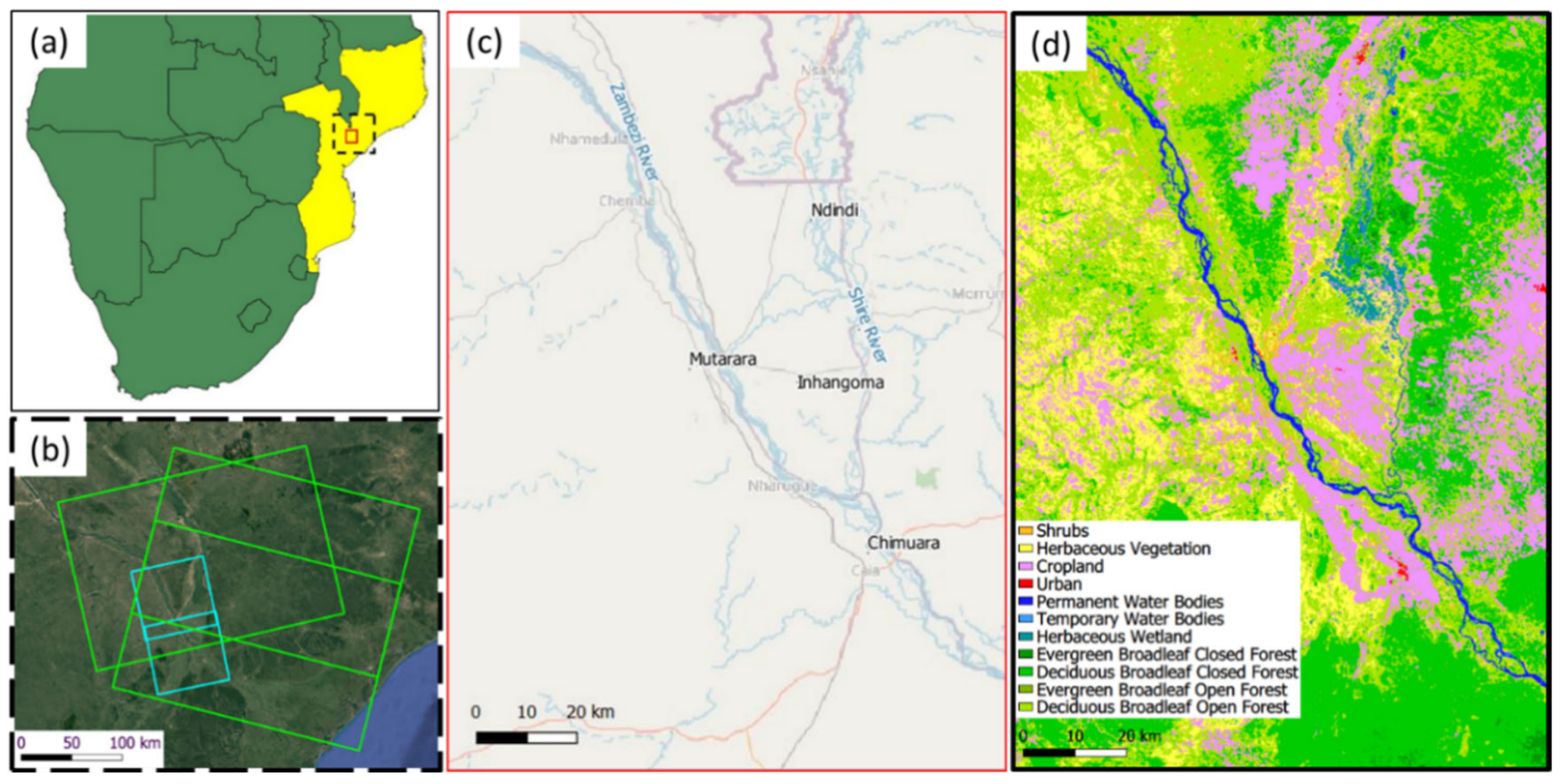
The basin, large about 1.4 million km2, is located in south-eastern Africa (Figure 1a) and spreads over eight countries (Angola, Botswana, Malawi, Mozambique, Namibia, Tanzania, Zambia, and Zimbabwe). The fluvial system is composed by the Zambezi River with its major tributaries (Congo, Cuando, Kafue, Luangwa, and Shire) and by the two dams of Kariba and Cahora Bassa. The course of the river can be divided into three main segments that represent different geomorphological units—Upper, Middle and Lower Zambezi—in which the river morphology changes in relation to the physiographic regions. Between the towns of Mutarara and Chimuara, the Lower Zambezi is characterized by the confluence with the main tributary, the Shire River, whose headwaters are in Lake Malawi. From the lake, the Shire River flows southwards, traversing gauges, rapids, and waterfalls until it forms a broad floodplain extending from Chikwawa to the confluence with the Zambezi, crossing the Elephant and Ndindi marshes and the Ilha de Inhangoma region. The latter, created by splitting the Zui Zui channel into the Shire River after a harmful flood in 1840, represents a region of interest, because recurrently subject to floods (Figure 1b). In fact, when the Zambezi is in flood, the (channeled) overflow pours into the Shire increasing its streamflow, until it exceeds and floods the valley [24]. This condition occurs with the reaching of peak flow (January–March) in the Zambezi and Shire rivers, during the wet season (November–April). The hydrology of the fluvial system, in fact, is determined by the seasonality of rainfall and water levels patterns, which, however, are conditioned by climate change and anthropic impact (flow regulation, i.e., dams) [23,25,26]. The variability of the natural processes (morphologic, hydrologic, and climate dynamics) has been modified strongly during the last decades, influencing the predictability of flood cycles and the consequent natural environment and anthropic landscape (villages, croplands, human activities, etc.) [27,28]. Moreover, as mentioned in the introduction, a variegated surface cover characterizes the area.
3. Materials
ALOS-2 PALSAR 2 (A2) and Sentinel-1 (S1) data were collected over adjacent, partially superposed orbits, in the dates and with the acquisition parameters listed in Table 1. Acquisition footprint locations are shown in Figure 1b. The two A2 scenes (two frames per date) are acquired in L band, in the FBD (Fine-Beam Double polarization) mode, in the HH and HV polarization channels, with ~10 × 10 m2 ground resolution, in ascending geometry. S1 images are acquired in C band, in the IW (Interferometric Wide-Swath) mode, in VV polarization, with 20 × 5 m2 (azimuth × range) resolution, in both ascending and descending geometries. Incidence angles are roughly comparable for all the used imagery, with 32° for A2 and 36° to 42° for S1 (S1 IW images have more than 15 degrees variation in incidence angle from ~30° at near to ~46° at far range: here we approximate the values for the selected area within the wide swath frame).
As can be seen from Table 1, one A2 acquisition is available on 9 February 2015, during the event, while one pre-flood image was acquired on 1 December 2014. S1 data are acquired with a 12-days repeat cycle in the period of interest. In our case, both ascending and descending acquisitions are considered, with intervals of 12 and 6 days. The higher frequency of acquisition of S1 images allows to better follow the event, with one acquisition in late January and 4 acquisitions in February 2015. One additional acquisition on 22 April 2015, is used as reference. All intensity images were calibrated, speckle filtered [29], geocoded and converted to dB scale.
We also use the CORINE land cover database [30], available at a resolution of 100 × 100 m2 over the African continent to interpret the backscattering evolution in time at different frequencies and polarizations. Although obtained by temporally averaged data from the Proba V satellite, such map contains sufficient information to characterize terrain typologies. The portion of the CORINE land cover map for the study area is shown in Figure 1c, with its standard color map legend.
All data were resampled to a ground resolution of 20 × 20 m2 through a nearest neighbor algorithm.
4. Methods
4.1. Preliminary Analysis—Detection of Open Floodwater as Decrease of Backscattering Value
One important aspect of flood monitoring is the possibility to follow an event in time. This is achievable at basin or larger scales through use of remotely sensed data acquired with high temporal frequency. SAR data are particularly sensitive to drops in microwave backscattering due to the presence of open water on the terrain surface. SAR data time series can be thus exploited, even in synergy with e.g., optical data [31], to compute multi-temporal maps illustrating the evolution of an event, such as the progressive draining of flooded areas, according to the topography and other hydraulic terrain characteristics [8,18].
Determining the extent of open water in a multi-temporal stack can be difficult when dealing with vegetated areas, as absolute backscatter drops may depend, e.g., on local conditions of wind or vegetation height. Several solutions have been proposed to retrieve reliably open water in time series of SAR images, relying, e.g., on harmonic analysis to model periodic flooding [7], or interpretation of backscatter time signatures [9]. We use clustering, a well-known methodology for data exploration and analysis. We adopt one of the best-known algorithms for data clustering, i.e., K-means. The K-means algorithm [32] iteratively assigns each element of a multi-dimensional feature space (the pixels’ backscatter values in our case), assumed Gaussian-distributed, to one among a pre-defined number of clusters, choosing the one with the shorter (Euclidean) distance, then recalculating cluster centers until convergence.
Here, we perform clustering of pixel backscatter values on the multi-temporal stack of images. We use a relatively large number of clusters (K = 32), to avoid neglecting small clusters of pixels with distinct behavior. We then inspect the retrieved clusters spatially and spectrally (i.e., the backscatter values of the cluster centers), to identify areas undergoing flood in each image. The clustering helps focusing on pixel sets which better follow expected backscatter change with respect to an unflooded image, neglecting other uninteresting typologies. This approach partly follows the core methodology delineated in the DAFNE algorithm [33], with a few differences. First of all, the automatic computation of prior probability values for the various clusters when L band signals are considered is not yet implemented in the DAFNE toolbox, so a heuristic procedure is used for this step. In fact, the experimental results here obtained can be considered as a useful study to opportunely integrate the software. Then, we do not have reliable ancillary data to precisely constrain spatially the flood phenomenon around the river course, as wetlands and other flooded terrain types are spread over a rather large surface in the river basin.
We here select the clusters with centroid values which best represent expected backscatter levels for each typology of flooded/non-flooded terrain, thus obtaining a multi-temporal representation of the flood evolution by considering areas inundated at different dates. Such multi-temporal flood maps are finally “classified” by assigning them to their corresponding CORINE class, in order to understand how the open floodwater is distributed over the different land cover classes.
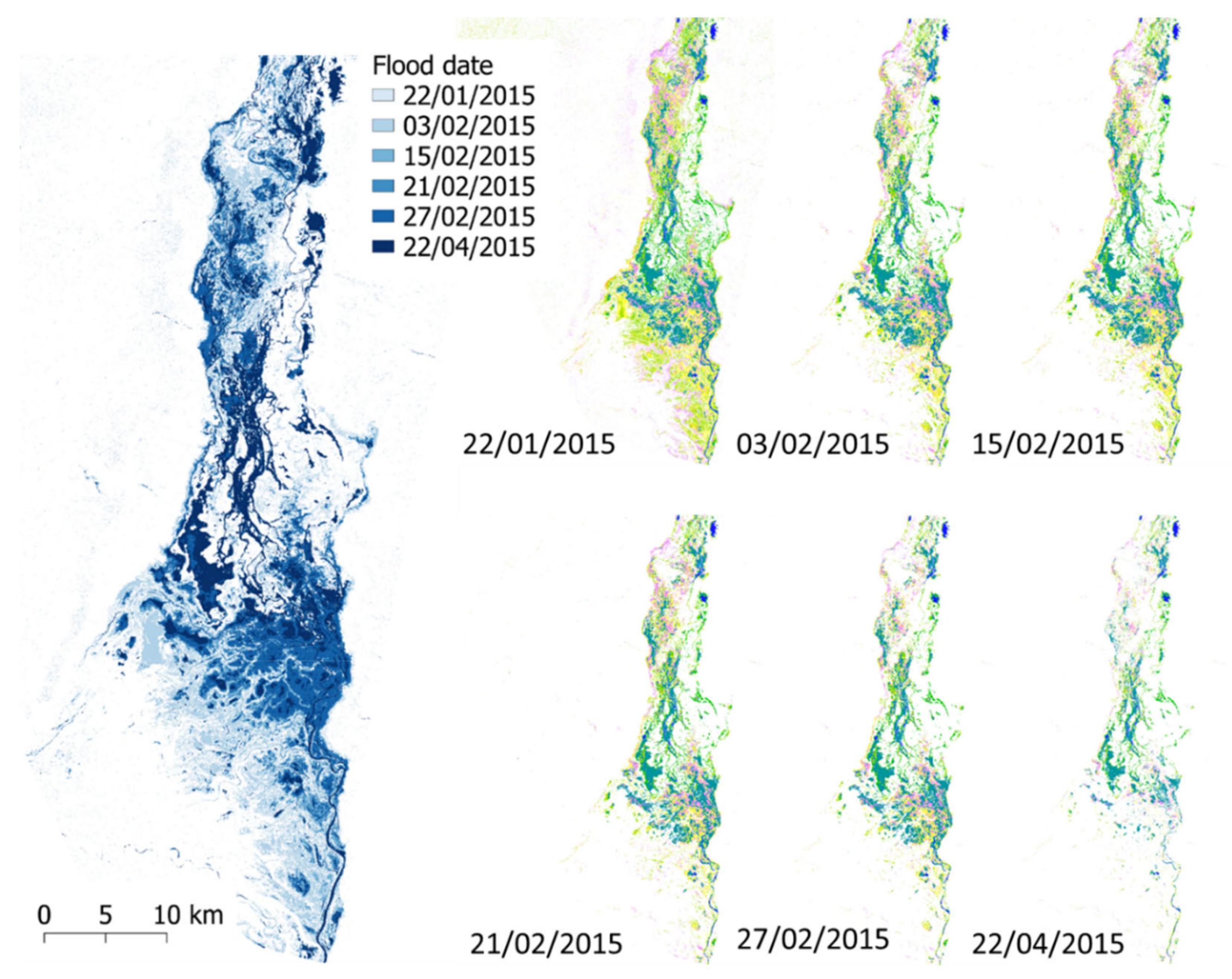
The left panel in Figure 2 shows the multi-temporal flood map obtained from S1 data. The map shows several areas around the main Shire river course, which are flooded only on the first imaged date of the event, i.e., 22 January 2015 (in light blue), and then gradually dry, so that smaller areas appear flooded from the first to each of the subsequent dates, from 3 February 2015 until 27 February 2015 (in darker blue tones). The darkest blue areas are those identified as water in the flood-free image acquired after the event, on 22 April 2015, taken as reference. Note that the Shire river course, clearly visible in the bottom part of the map, appears correctly in dark blue.
The right panels show the six successive flood maps derived from the S1 acquisitions, colored according to the underlying CORINE land cover classes, reported in the legend in Figure 1. It can be seen that the largest flooded area, in the first date, covers several class types, spanning cropland (pink pixels, spread throughout the whole region), herbaceous wetlands (blue-green areas at the center/bottom), all four types of broadleaf forest (evergreen/deciduous, open/closed, corresponding to different shades of green, present especially close to the center-right of the area), and herbaceous vegetation (yellow areas mostly in the bottom-left). As the flooded area shrinks, in the following dates, it affects less and less herbaceous vegetation and cropland, leaving mostly wetlands and a few forested areas as flooded in the last date.
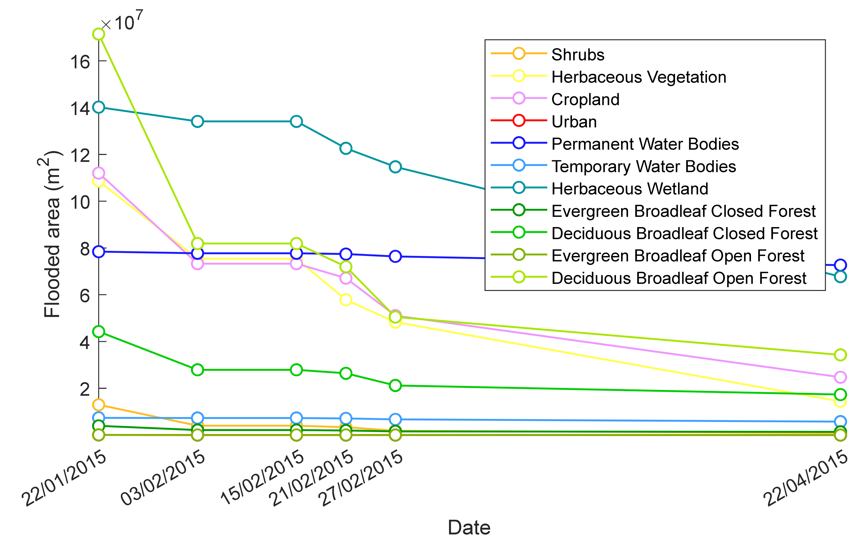
This is confirmed by analyzing quantitatively the number of pixels detected as (open-water) flood in each CORINE class, for each of the S1 acquisitions, as reported in Figure 3 It can be seen how, on the first event date, the CORINE class most affected by flood is the Deciduous Broadleaf Open Forest, followed by Wetlands, Cropland, and Herbaceous Vegetation. The quantity of flooded pixels in the Deciduous Broadleaf Open Forest class decreases, during the evolution of the event, to approximately 1/5 at the end of the period. Herbaceous Wetland pixels are the second most populated class in the first date, but they become the first one from the second date onward. Cropland, Herbaceous Vegetation and Deciduous Broadleaf Open Forest all show similar decreasing trends, while Deciduous Broadleaf Close Forest shows smaller areas throughout the whole imaged period. Other classes appear more marginally affected. Notably, the areal extent of both the Permanent and Temporary Water Bodies classes remain practically constant throughout the event, thus qualitatively confirming the consistency of the analysis.
It can be noticed that many areas at the center-right of the maps in Figure 2 appear not flooded in any of the acquisition dates, thus looking like “holes” in the maps. By looking at the overall CORINE map in Figure 1b, these appear to correspond mostly to forested areas. This observation is thus compatible with the interpretation that C-band radiation is not able to penetrate thick (“closed”, in the CORINE terminology) forest cover. However, many of the closed forest undetected areas appear to be spatially close, or even surrounded, by areas detected as flooded. As no significant topography is present in the area, it is presumable that at least part of these forested areas are indeed flooded beneath the canopy, although C-band microwaves cannot “see” through the thick forest stands.
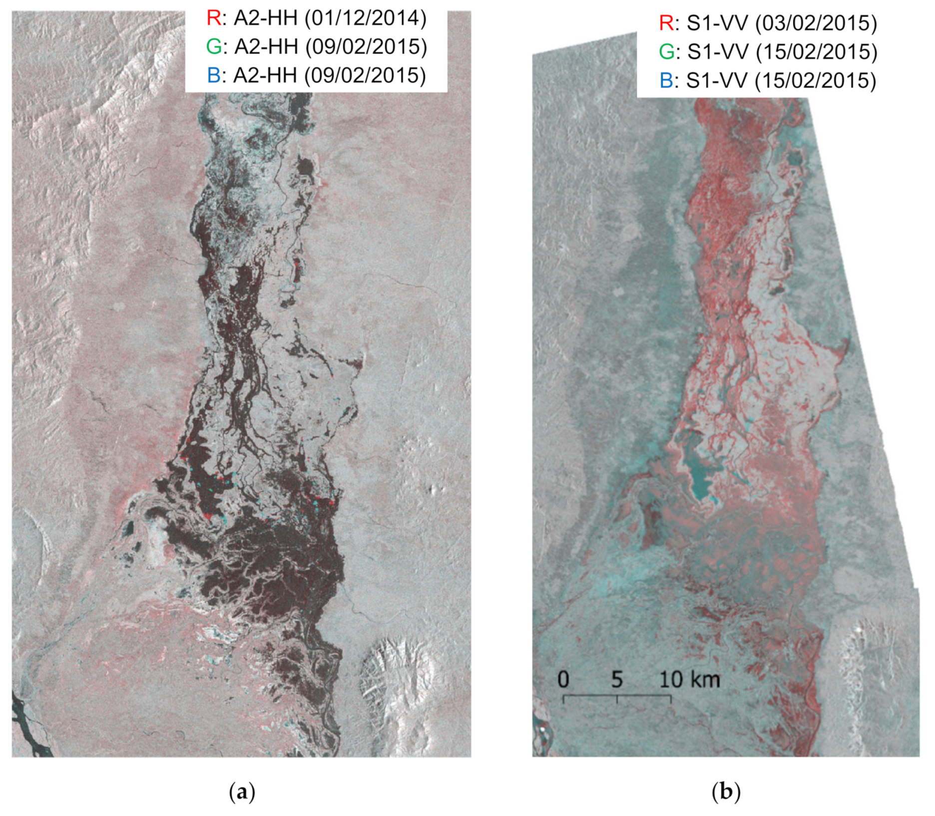
One last observation about the C-band multi-temporal analysis is that, as appears in both the maps in Figure 2 and the plots in Figure 3, the flooded area between 3 and 15 February 2015 appears identical. In our K-means clustering analysis, this comes from the fact that it was not possible to determine statistically significant pixel clusters showing different flood behavior on these two dates. In fact, an RGB combination of the two Sentinel-1 intensity images acquired on 3 February 2015 (red channel) and 15 February2015 (green and blue channel), reported in Figure 6a below, shows that very little appears to change from one date to the other, as very few red or cyan colored pixels are visible within the area interested by the flood. This allows to confirm empirically that, between these two dates, the situation on the ground is substantially stationary, as suggested by the previous multi-temporal analysis. As a consequence, the available A2 image, acquired on 9 February 2015, can be investigated in synergy with one of the two S1 acquisitions, treating the S1-A2 imagery as a multi-frequency dataset referred essentially to the same snapshot in time. This is investigated in Section 4.2 below.
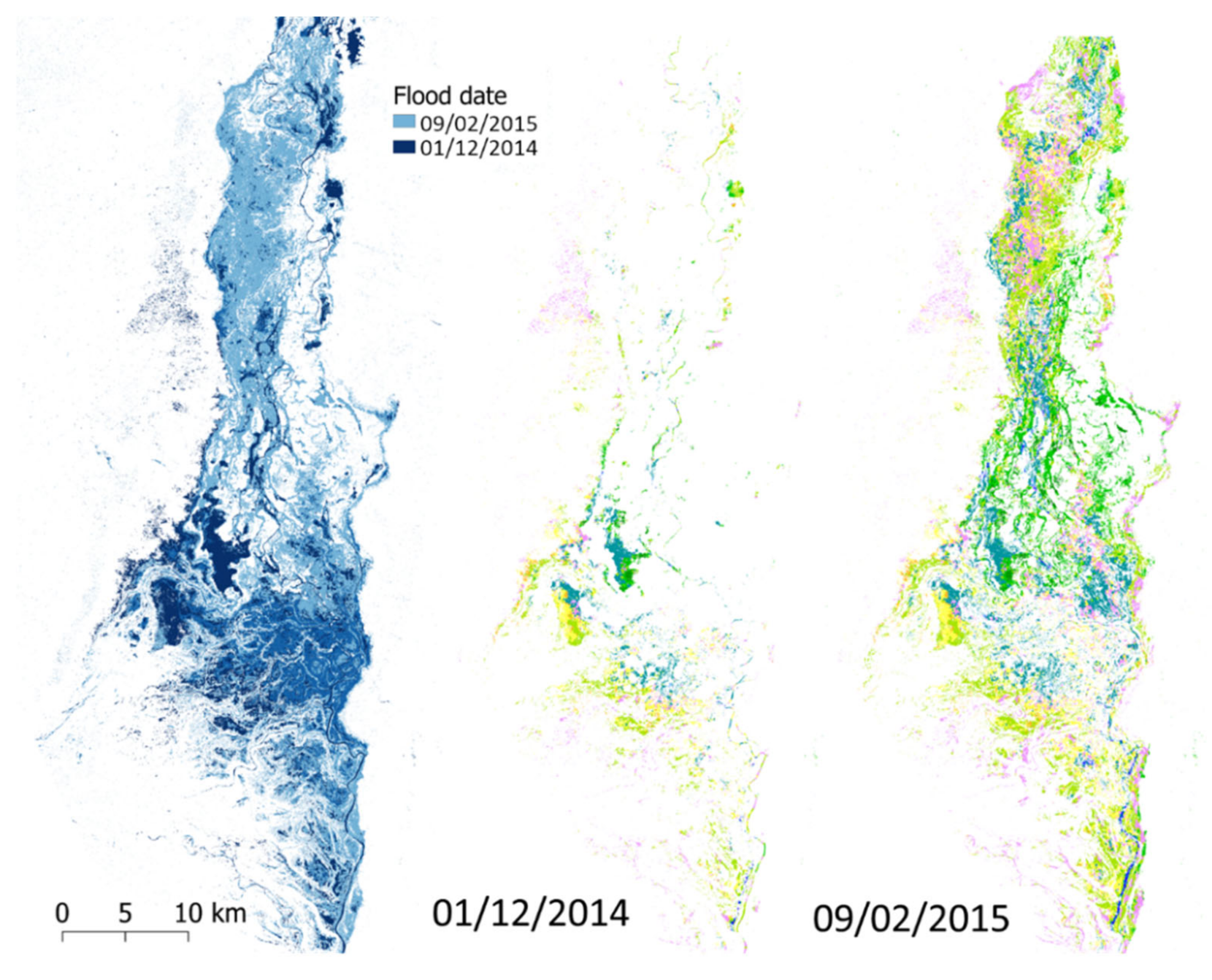
The same analysis as the one just presented on C-band data has been performed for the L-band stack, composed by only two images, one acquired before and one during the flood event. In this case, analysis is limited to the “permanent water” areas detected in the pre-event image, and the open water areas in the single co-event image. Figure 4 shows on the left the multi-temporal map in the same color code as the one on the left of Figure 2, and on the right the two maps corresponding to the two dates, with each pixel classified and colored according to the corresponding CORINE map. By comparing the multi-temporal maps in Figure 2 and Figure 4, some differences can be noticed. First of all, as expected, the multi-temporal map obtained from A2 data appears slightly more “dense” (i.e., with less empty areas) in the central part of the basin with respect to that obtained from S1.
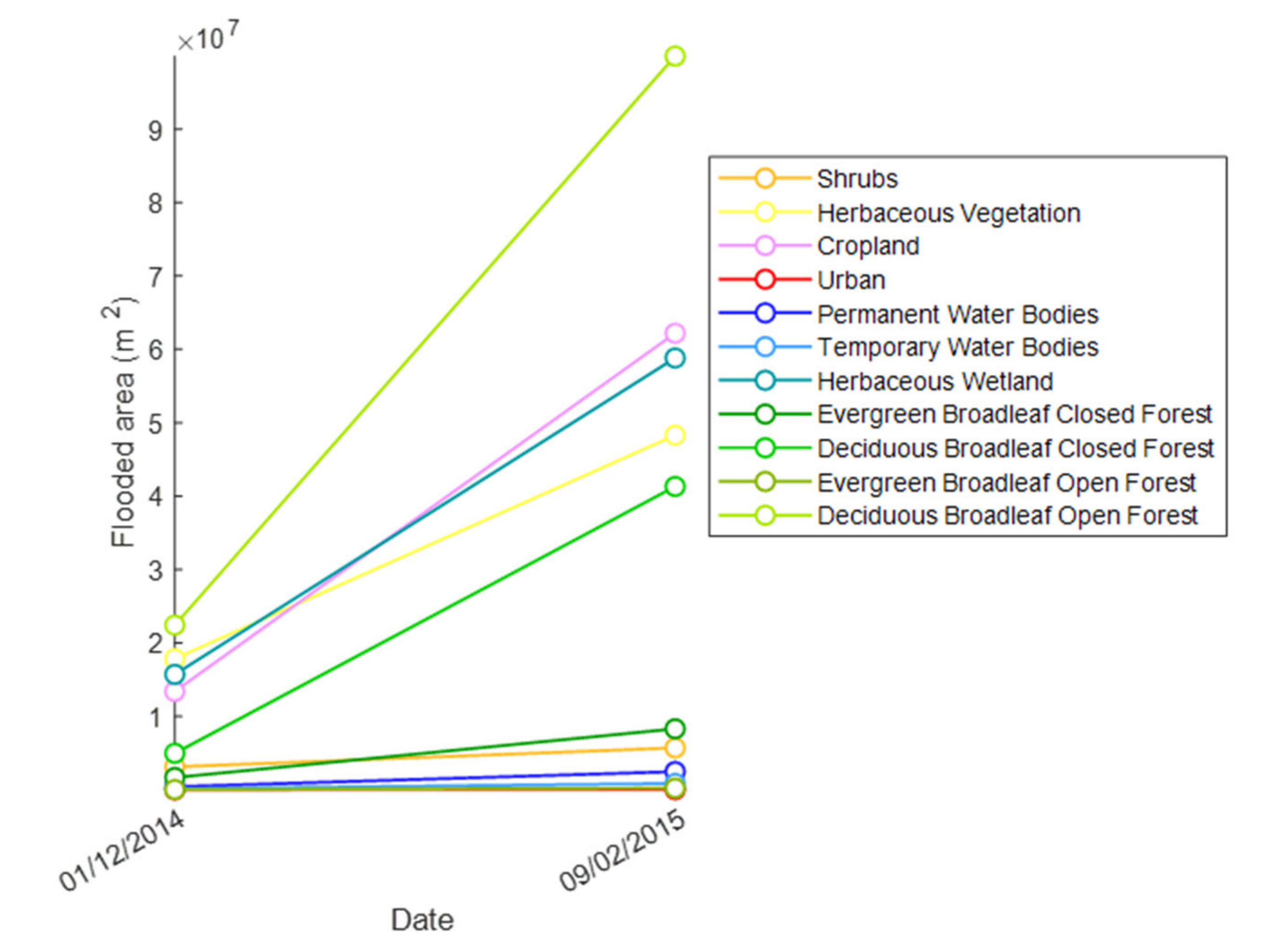
Another observation concerns the distribution of land cover classes affected by the flood in the two cases. As noted above, S1 data allow to conclude that the situation on the ground between the dates of 3 and 15 February is substantially the same; nevertheless, the flood map realized from A2 data, dated 9 February (the rightmost map in Figure 4), appears to have different quantities of yellow (corresponding to herbaceous vegetation), pink (corresponding to crops) and light green (deciduous open forest) pixels than the corresponding ones from S1. This is confirmed by looking at the estimated areas covered by open flood water for each CORINE class in the two A2 dates, reported in Figure 5. A higher area covered by open forest can be noticed, and at the same time smaller areas corresponding to herbaceous vegetation and cropland. This comparison, taking for valid the assumption of stationary ground situation between the two dates of 3 and 15 February, shows that the interaction and backscattering of L-band microwaves with flooded terrain is slightly but significantly different than that pertaining to C-band radiation.
To further delve in this matter, in Figure 6b we show a RGB combination of the SAR backscatter of the A2 (HH) images acquired on 1 December 2014 (red channel), and on 9 February 2015 (green and blue channels): as can be seen, some groups of red pixels, which are the areas exhibiting lowering of backscatter in L band, correspond to the ones which are dark in Figure 6a, i.e., open flood water in both the co-event C-band images. However, some cyan areas are also visible in correspondence of C-band dark areas. Moreover, some areas in the lower-left part of the basin appear bright in C band (panel a) and dark in L band (panel b). These large differences between the two images confirm the presence of areas with different penetration and thus different microwave interaction in images from the two sensors.
4.2. Statistical Multi-Sensor Backscatter Analysis of Land Cover Classes
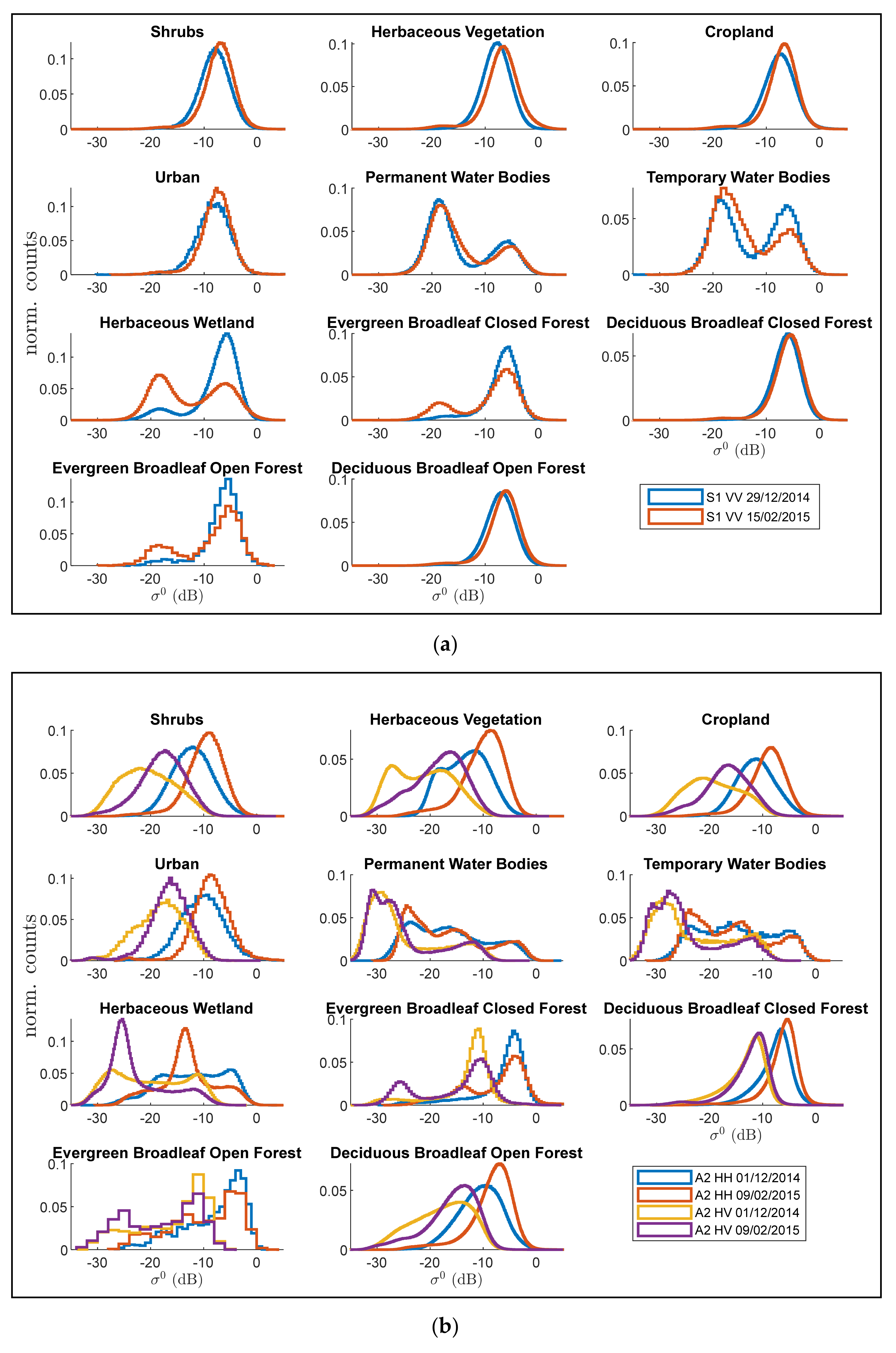
We now adopt the dataset shown in red color in Table 1, which includes one pre-event and one co-event image for each type, one S1 pair in VV polarization, and two A2 pairs in HH and HV polarizations, respectively, as a multi-sensor stack referring to the same situation on the ground. To gain some further insight into the different types of land cover present on the ground, we analyze statistically the backscatter signatures of the various CORINE land cover classes. In Figure 7 we report the histograms of the SAR intensities for pixels belonging to the land cover classes present over the area, selected by using masks obtained by the CORINE map.
As can be seen, Shrubs and Cropland exhibit a slight increase of backscatter (the peaks move to higher values) from pre- to co-event imagery in C band (up to 1 dB), but a more consistent one in L band (3–5 dB). This could be due to the presence of double bounce effects in flood conditions, which is known to increase backscatter up to several dB. A moderate increase of backscatter (peaks shift of about 1 dB in both bands) is also detected on the Urban class, although sample population is much reduced in this case. Deciduous Broadleaf Open and Closed Forest classes exhibit a less uniform behavior, with an appreciable increase registered only in L band and HH polarization (A2-HH), while in both L-band HV and C-band VV images, the intensity distributions do not change consistently. Open forest seems to exhibit smaller secondary peaks at very low backscatter levels (approximately between −20 and −25 dB), possibly corresponding to flooded forest patches. Similar lower secondary peaks are just barely visible in pixels corresponding to closed forest, as could be expected from a lower penetration of the thicker canopy.
Some types of land cover exhibit clearly bimodal intensity distributions in at least some of the SAR image bands. This is evident for classes such as Herbaceous Vegetation (in L band), and Herbaceous Wetland (in both bands). The former exhibits just a small (~1 dB) increase in the peak backscatter value in C band; in L band, pre-flood backscatter exhibits a peak at very low values in both polarizations, as well as a second one at higher values, while in co-event images the first peak appears much lower, and the secondary peak shifts up by 2–3 dB. The latter (Herbaceous Wetland) exhibits a clear increase in the low-intensity peak in C band from pre- to co-event data; in L band, both polarizations show a consistent increase and a small shift of the low-intensity peak from pre- to co-event. Both Open and Closed Evergreen Broadleaf Forest show bimodal histograms in co-event images, while pre-event data show very small to null low-intensity peaks.
Bi- or sometimes tri-modality can also be observed for Permanent and Temporary Water Bodies, with small shifts from pre- to co-event conditions. The presence of several peaks is likely due to the lower resolution of the CORINE data with respect to the SAR ones, so that many pixels falling in the Permanent/Temporary Water Bodies CORINE class (mostly located on and around the river course) actually correspond to other land cover classes on the ground; the lower peak in C-band VV backscatter seems to correspond to two separate peaks in L-band HH data, while L-band HV is still bimodal, although with distributions shifted by −6/−10 dB.
These results already confirm a consistent increase in information brought about by the use of multi-frequency data. As is often the case, especially for remote regions such as those in African countries, where validation or updating campaigns are difficult, the land cover map may contain some difference with respect to the actual situation on the ground. To further refine our inference, we analyze in higher detail the S1-A2 integrated multi-frequency dataset.
4.3. Multi-Frequency and Multi-Polarization Floodwater Mapping
As mentioned above, the backscattering properties of terrain surfaces, as well as their changes due to inundation events, depend on the wavelength of the radar sensor. In thickly vegetated areas, floods may affect different types of ground environments, exhibiting different vegetation densities and other terrain properties, so that detecting exhaustively floodwater in such cases can be difficult. For instance, it is important to be able to detect flooded vegetation, besides open water areas. This is possible thanks to the so-called double bounce phenomenon, in which microwaves can be scattered back towards the sensors after bouncing on the surface and the vertical vegetation structures (tree trunks or plant stems). In other cases, more sparse and thin vegetation, such as grass or shrubs, may appear darker when flooded in SAR images acquired at longer wavelengths, as the diffusion effect of the canopy is weaker. Vice versa, shorter wavelengths may give rise to enhanced backscatter from such vegetation in flood conditions.
After the preliminary analyses described in the previous sections, we are now ready to use the complementarity of the A2 L-band image acquired during the flood, with both its polarization channels (HH-HV), and the S1 C-band one, to gain some further insight into the different types of land cover present on the ground and their backscattering response in presence of floodwaters, thanks to the multi-frequency (and multi-polarization) stack of C- (VV) and L-band (HH and HV) pre- and co-flood image built in the previous sections. This stack presents a variety of behaviors, including backscatter decrease and increase for various vegetation types and flood conditions, caused by phenomena such as specular reflection, double bounce, or wind. To better interpret such huge wealth of information, this stack is again processed through K-means with a number of clusters sufficient to isolate backscatter change signatures. The number of clusters is then reduced through a merging procedure which iteratively joins the two clusters with minimum Battachaarya distance. Finally, the most interesting clusters are interpreted by comparing their signatures and change with the CORINE land cover information. The algorithm is thus composed by the following steps:
- Full data stack (multi-temporal, -frequency, and -polarization) clustering, where the first guess for clusters number is the double of land cover classes available. In our case, the number of available classes is provided by CORINE land cover map and each class is assumed to be flooded or non-flooded. The only exception is the permanent water class that cannot change its state during the flood event.
- Clusters number reduction.
- Classification of each cluster based on the mean values of input features and the dominant land cover class.
5. Results
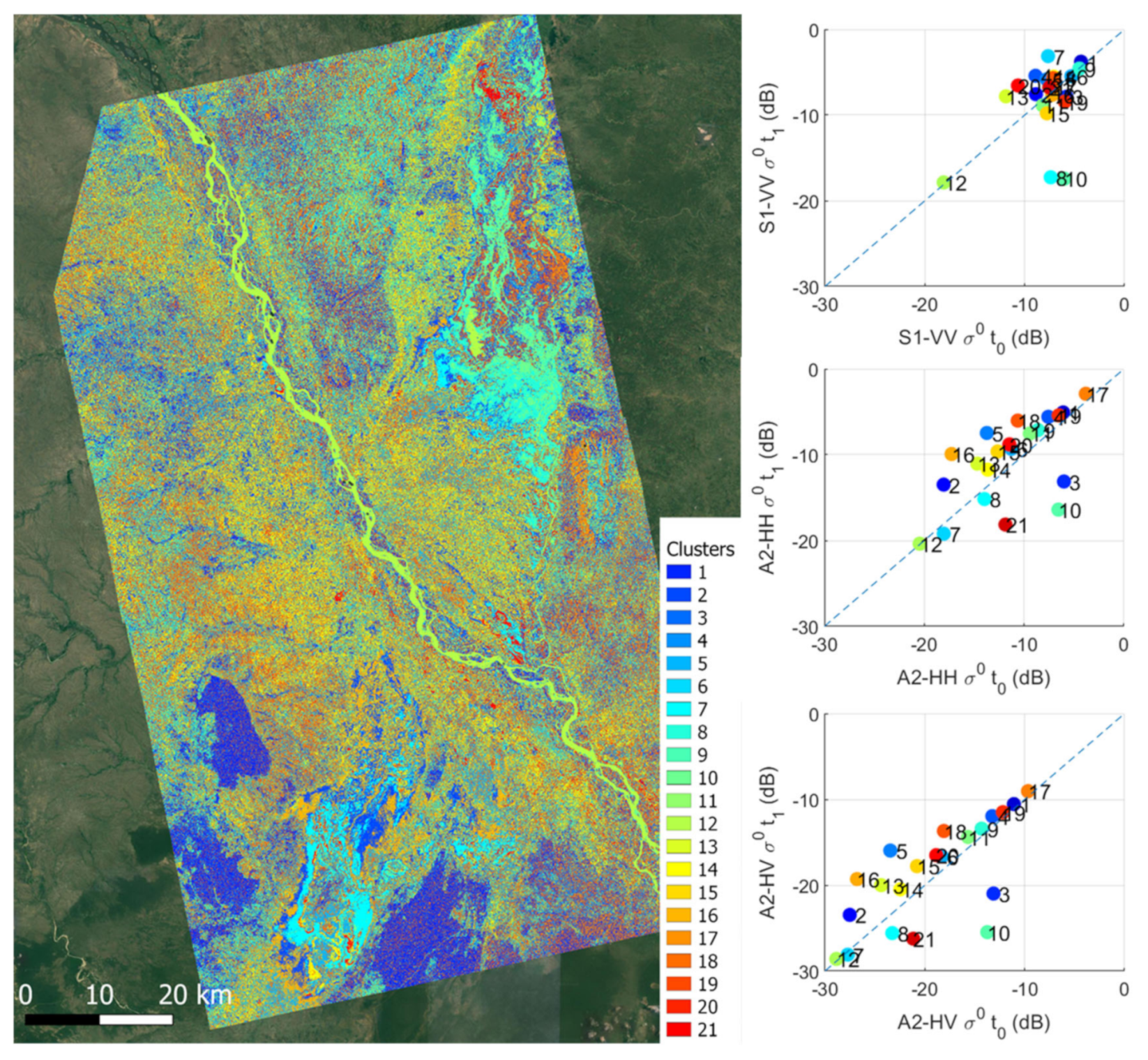
As described above, our data are arranged in a 6-dimensional array, containing the six SAR intensities corresponding to the entries in red in Table 1. We begin our analysis by heuristically choosing a number of clusters equal to 21, which corresponds to the number of CORINE classes present on the area (11), considered in both flooded and unflooded conditions, with the obvious exception of permanent water areas.
Figure 8 shows a map of the clustered image, spanning the whole area covered by the image frames, where pixels clusters are represented in different colors. To ease interpretation, 3 scatter plots are also shown in the figure, showing the 21 cluster center positions in each of the 3 planes spanned by the pre-flood and the flood backscatter values in each channel (indicated as times and , respectively). As can be seen, the map shows some cluster centers which appear relatively compact spatially, while others are more scattered throughout the area. In the scatter plots, cluster centers which fall farther from the main diagonal (shown as a dashed line in each plot) exhibit the most interesting behaviors.
Some cluster centers appear above the scatter plots’ diagonals, at least in some cases. These are likely to correspond to double bounce phenomena due to flooded vegetation, leading to increased backscatter in one or more channels. It appears, however, that many cluster centers of this kind are very close to each other, suggesting their possible belonging to the same class on the ground. In practice, it appears that the postulated initial number of clusters (21) is too high with respect to what can be actually distinguished in the data, and thus a lower number may be more acceptable. However, which one is the best? The choice of the most suitable cluster number is a long-standing problem in data analysis, and several methods have been developed to deal with it. A common practice is to start from a relatively large number of clusters, then merge “close” clusters iteratively, according to some distance measure, until satisfying some quality criterion. Such a hierarchical approach has been adopted, e.g., in [34], by using available ground truth as a reference. Here, we adopt a similar approach, stopping the clustering procedure when a heuristic criterion of homogeneity is reached.
We proceed as follows: starting from the maximum number of clusters (21 in this case), we merge together the two clusters which have the smallest Bhattacharyya distance [35] from each other, iterating the process until being left with only two clusters encompassing the whole dataset. At each iteration, we re-compute the coordinates of the cluster centers (as average of the coordinates of the points belonging to that cluster).
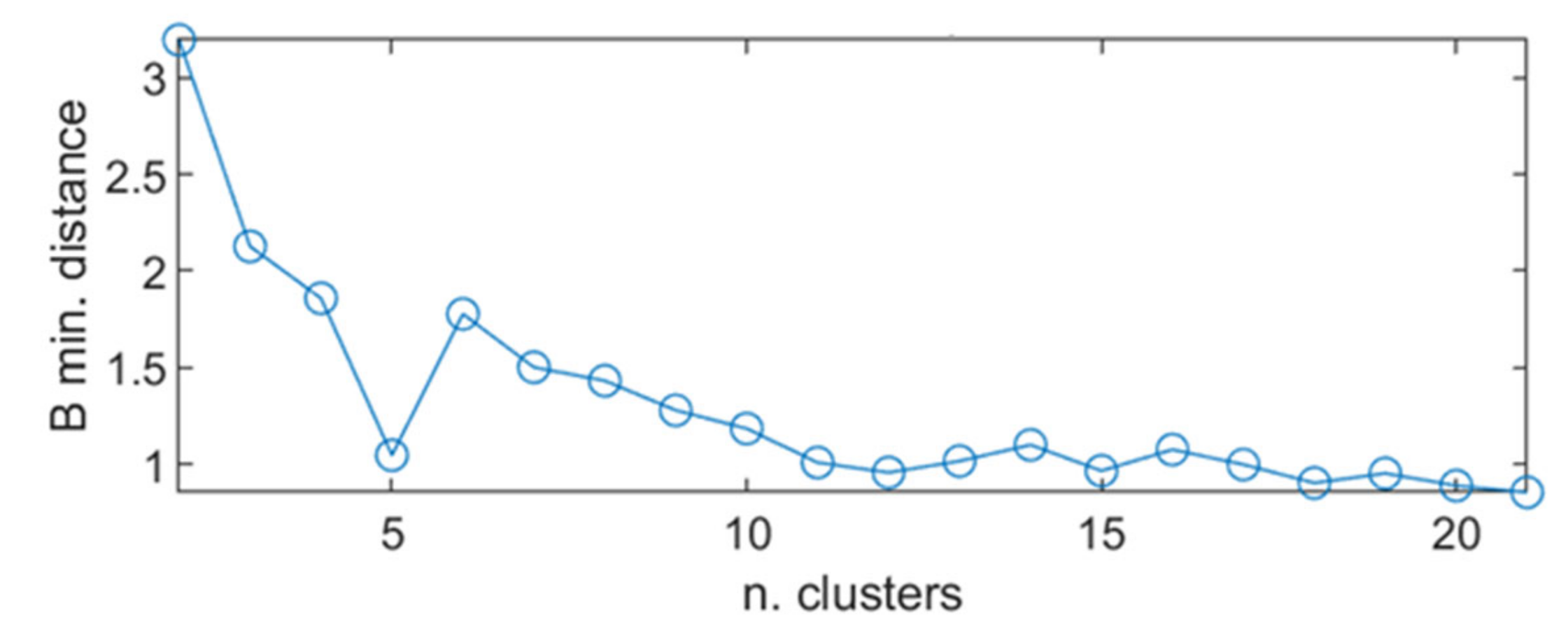
In Figure 9 we show the minimum Bhattacharyya distance computed between the various clusters, as a function of the number of clusters. The measure stays relatively constant as clusters are decreased from 21 to about 12 (moving from right to left in the plot), then has a general increasing trend as clusters are reduced further, with some fluctuations, reaching the maximum value for just 2 clusters. We take the position of the approximate discontinuity in the trend described above as the “optimal” value, through the following reasoning: while pairing clusters above the “optimal” number, the minimum distance is only slightly affected—i.e., we are likely merging bulks of very close clusters. As the last cluster of these bulks is merged with its closest member, then larger distances begin to be left in the data, and thus the minimum Bhattacharyya distance increases. So, our “optimal” cluster number is the one after which the minimum distance begins to increase appreciably. This corresponds, in our case, to the number of 12 clusters.
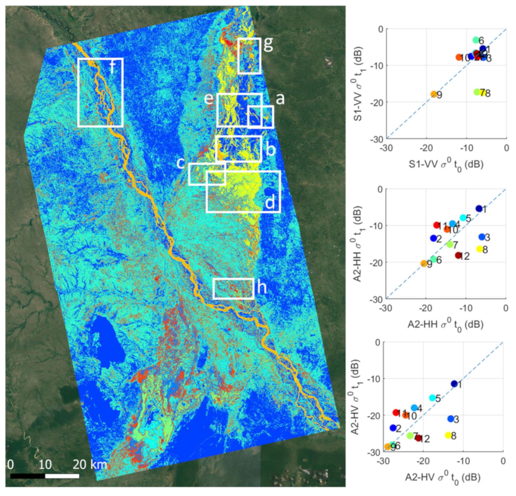
Figure 10 then shows the corresponding clustered map, together with the same scatter plots as in Figure 8, for this “optimal” number of 12 clusters. Here, more uniformly spaced cluster centers are visible. In addition to those corresponding to permanent water (n.9 in this case), and open water flooded areas (n.8), we notice cluster n. 11, which corresponds to an increase of about 8 dB in L band, while exhibiting no significant change in C band, so likely corresponding to forested areas with thick canopy layer, which can be penetrated by lower frequency electromagnetic waves, thus causing double bounce with the bottom water layer, but not by C-band radiation.
This cluster is represented in bright red and appears in the top part of the map on the left of Figure 10, corresponding loosely to forest classes in the CORINE database. A similar behavior, although with lower intensity increases (up to a maximum of 3–4 dB) can be discerned for clusters n. 2, 4, and 10. A rather peculiar behavior is shown by cluster n. 6, in cyan-greenish color, which exhibits an increase of about 4–5 dB in C band, while staying very close to the diagonal, with rather low backscatter values at both times, in L band. This class, located in a rather compact area at the center of the map, likely corresponds to shrubs or low, thin vegetation, causing likely an increase in C-band backscatter, while resulting “transparent” to longer wavelength radiation.
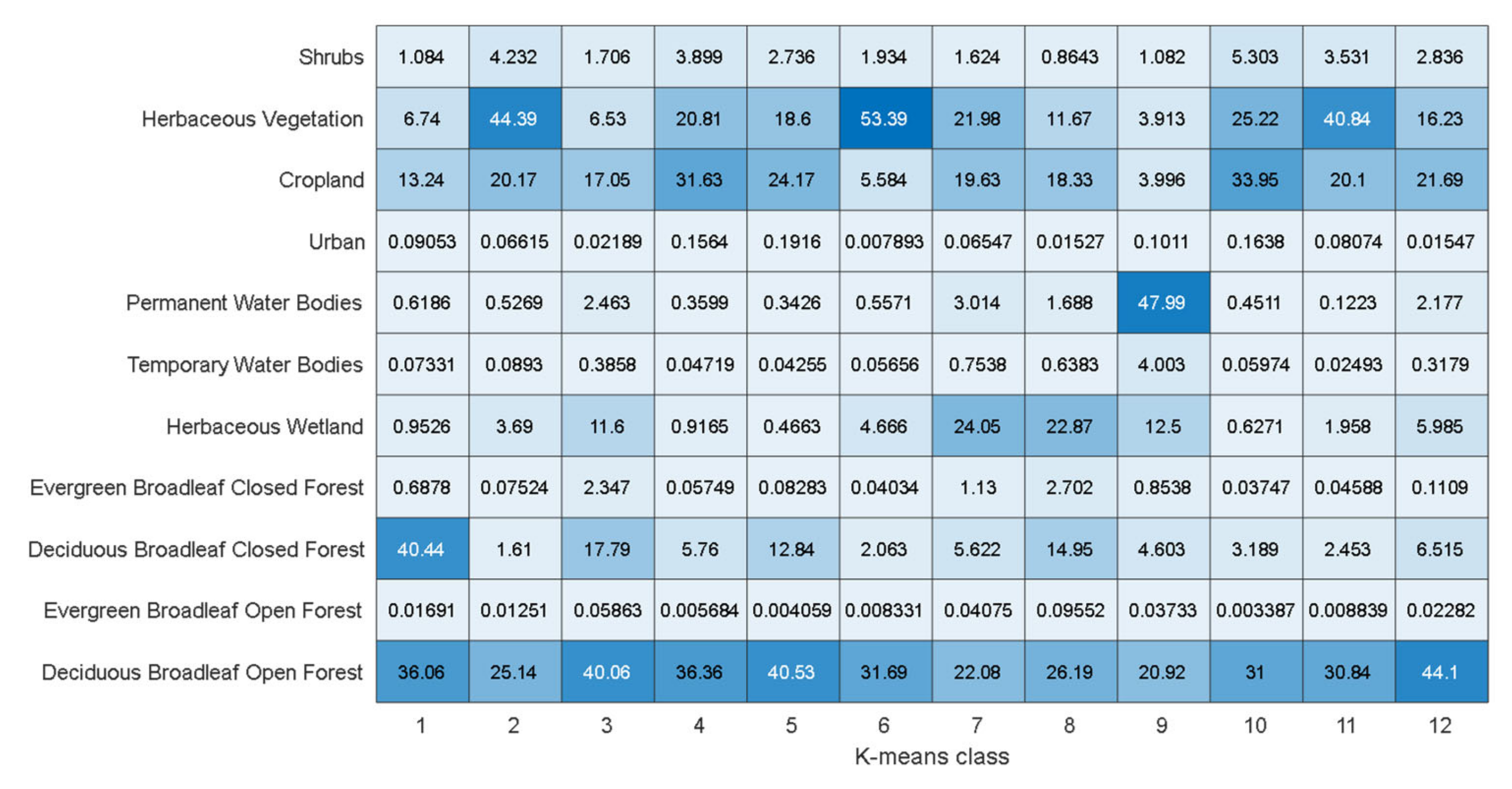
Figure 11 illustrates the correspondence of the 12 clusters with the classes in the CORINE land cover map. Each entry in the matrix represents the percentage of pixels belonging to a given cluster (columns) and a given CORINE class (rows). This matrix offers some additional indication about the clustering results. In the following, we present an integrated interpretation of the types of response of each cluster with respect to the corresponding land cover CORINE classes.
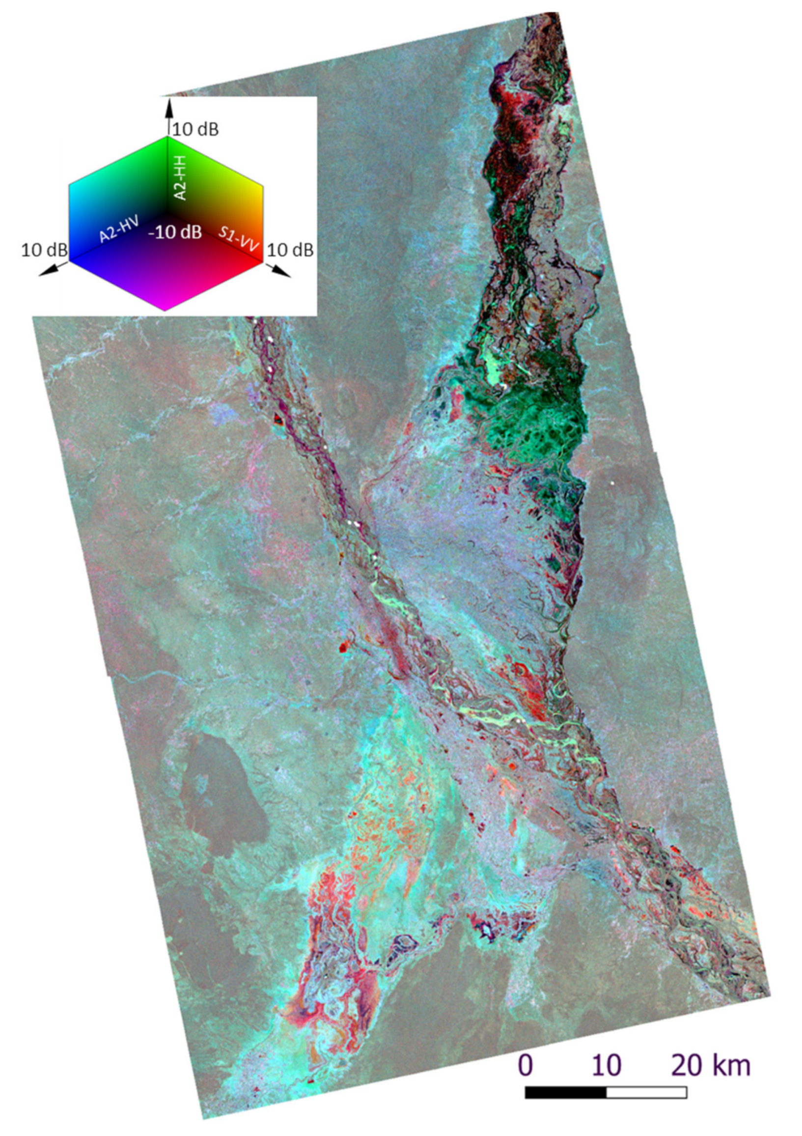
To improve the visual representation of local spatial support of the backscatter signatures, we also consider a RGB combination of the three ratios between co- and pre-event SAR, red for the S1-VV, green for the A2-HH, and blue for the A2-HV (Figure 12). The different speckle patterns in the three channels give this image a somewhat smoother appearance than single SAR images, so we use the color in this image as an aid to detect and interpret the multifrequency type of backscatter with respect to the land cover. Generally, in the change RGB image in Figure 12, black areas underwent strong backscatter decrease (colors are saturated at ±10 dB for better contrast visualization, as shown in the figure inset color cube) in all three channels, likely corresponding to open water; dark red corresponds to decreasing backscatter in L-HH/HV imagery, while maintaining roughly constant levels in C-VV. This would likely correspond to vegetation with a structure which allows penetration of longer wavelengths (L band), which therefore undergoes specular reflection, while C-band waves are backscattered by the canopy, and therefore do not exhibit significant changes when flooded. Dark green pixels underwent backscatter decrease in L-HV and C-VV, while keeping roughly constant values in L-HH. This could be due to different wind conditions on the two acquisition dates (3 and 9 February 2015 for A2 and S1, respectively), which cause the water surface to backscatter more power in the second date (in L-band) than in the first one (in C-band). The higher change in HH than in HV polarization also suggests this kind of explanation, since cross-polarized channels are reported to be less sensitive, in terms of backscatter, to rough surfaces such as water interested by capillary waves. Notably, the opposite behavior (decreasing HH, constant HV channels), which would correspond to dark blue pixels, is not seen on the image.
In contrast, bright colors denote increase (positive change) in backscatter levels, hinting to the possible presence of flooded vegetation or other structures with double bounce behavior. For instance, on bright red areas, C-VV backscatter increases, while both L-HH and L-HV decrease. These may correspond to short vegetation, such as shrubs, herbaceous vegetation, or cropland, where shorter wavelengths experience double bounce by the interaction of stems/leaves and the underlying water surface, more than longer wavelengths. Vice versa, bright green and cyan areas denote increase in both L-HH and L-HV channels, respectively, with decrease or no change in C-VV. These may indicate the presence of flooded forest or wetlands, where tree trunks or other thick structures contribute to backscattering of longer wavelengths.
These considerations seem confirmed by comparing the RGB-backscatter ratio map with the indicative CORINE land cover map. In the following, we discuss each of the detail areas highlighted by white rectangles in Figure 10 integrating information from multiple sources. The discussion is presented for each of the clusters corresponding to flooded areas.
6. Discussion
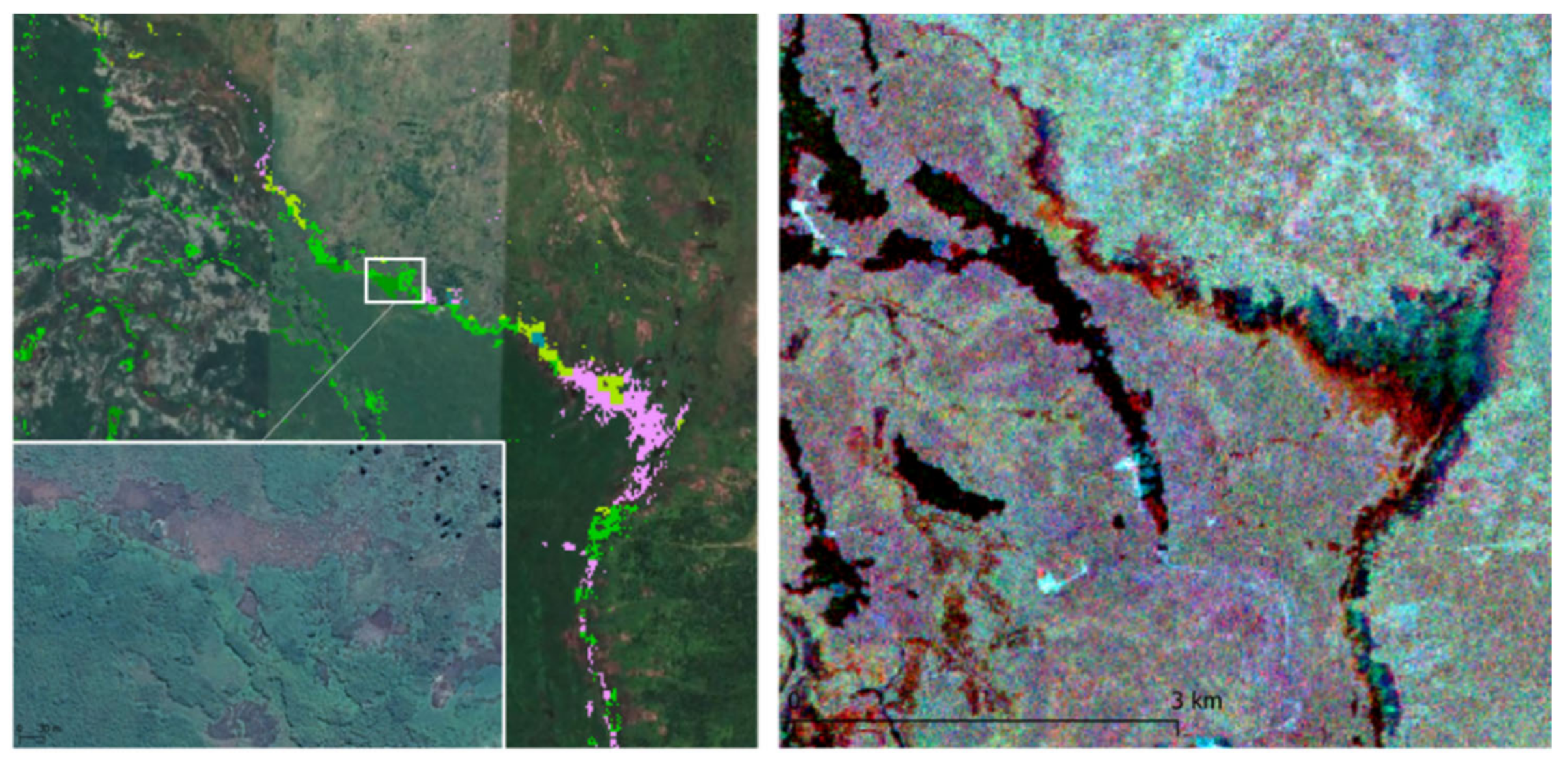
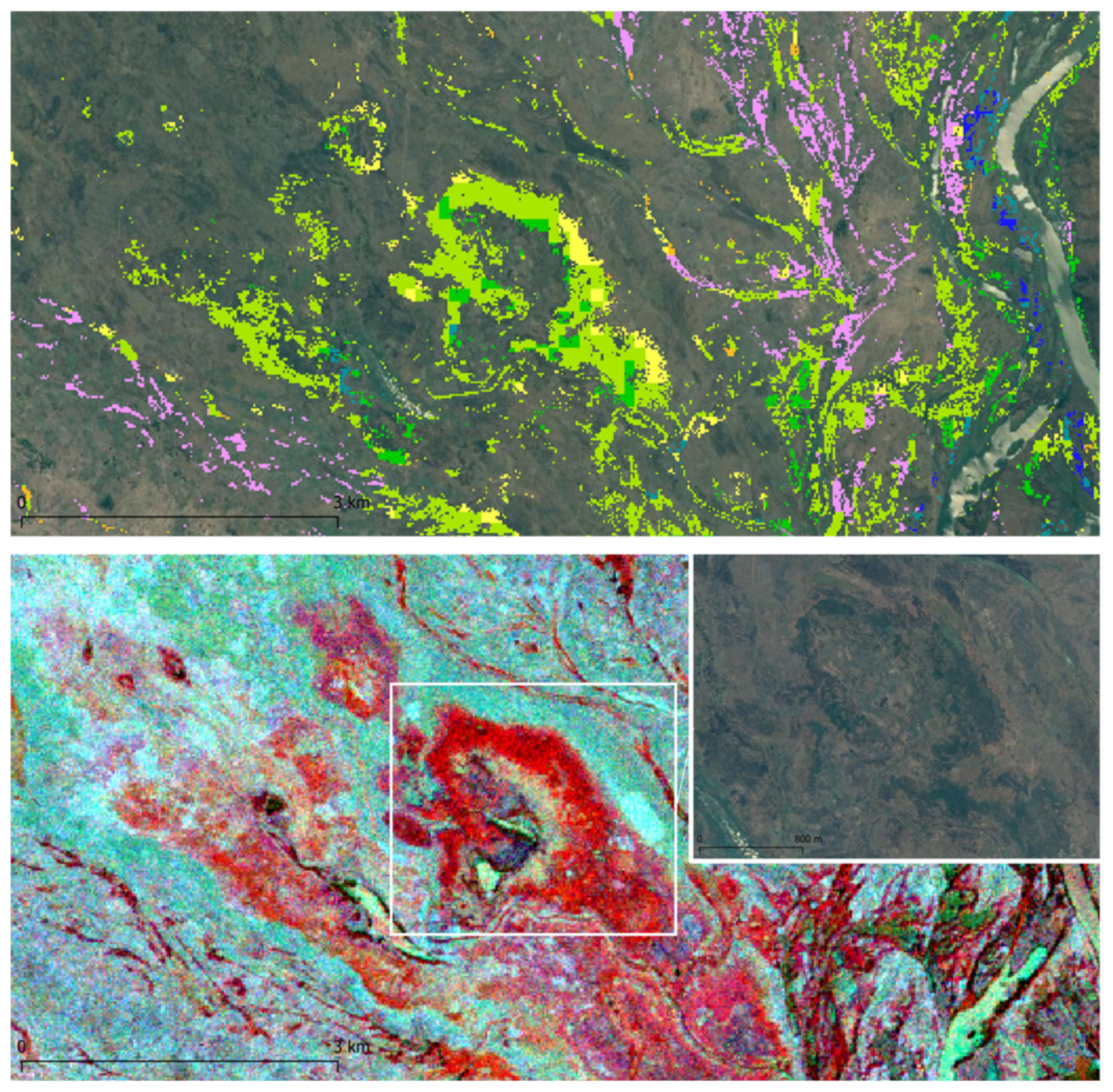
Cluster 3 is composed of pixels falling mostly (about 40%) in the class Deciduous Broadleaf Open Forest (Figure 11), with lower percentages of Deciduous Broadleaf Closed Forest and Cropland (both about 17%). Its center backscatter exhibits consistent decrease in L-band data (about 7 dB), but a negligible decrease (about 1 dB) in C-band. The example in Figure 13 shows a spatial localization of this cluster at the border of a thickly vegetated area. The strong decrease in L-band backscatter indicates the presence of open water, while the C-band response seems to be that of a vegetated canopy. The detail inset on the bottom-left of the figure shows a forest glade, which corresponds to pixels in this cluster. Most of these areas seem in fact to correspond to clearings in the forest canopy, exposing the underlying surface, likely covered by low vegetation. During the flood, such clearings can be penetrated by L-band radiation, thus causing the darkening, but not by C-band shorter wavelengths.
Figure 14 shows, at the top, pixels corresponding to clusters 4 and 5, colored according to the CORINE class legend. These clusters exhibit similar compositions in terms of CORINE land cover classes on the ground, with 36 to 40% of Deciduous Broadleaf Open Forest, 24 to 32% of Cropland, and 18–20% of Herbaceous Vegetation (Figure 11). The cluster center coordinates in the 6-dimensional backscatter space correspond to roughly constant levels in C band, around −7 to −8 dB, and a slight increase of about 3 dB in L band. The spatial support of this cluster is rather large, corresponding to a relatively large variance of its components. Nevertheless, it includes locally some spatially compact areas, such as those shown in Figure 14. The corresponding RGB image at the bottom of the figure shows the correspondence of the cluster pixels with bright blue/white areas, corresponding to rather strong backscatter increase in both HH and HV L-band, or even in all three channels. The detail inset highlights the different texture in the forest canopy cover corresponding to the cluster pixels, indicating the likely occurrence of more open forest stands, allowing double-bounce phenomena when floodwater is present below the canopy.
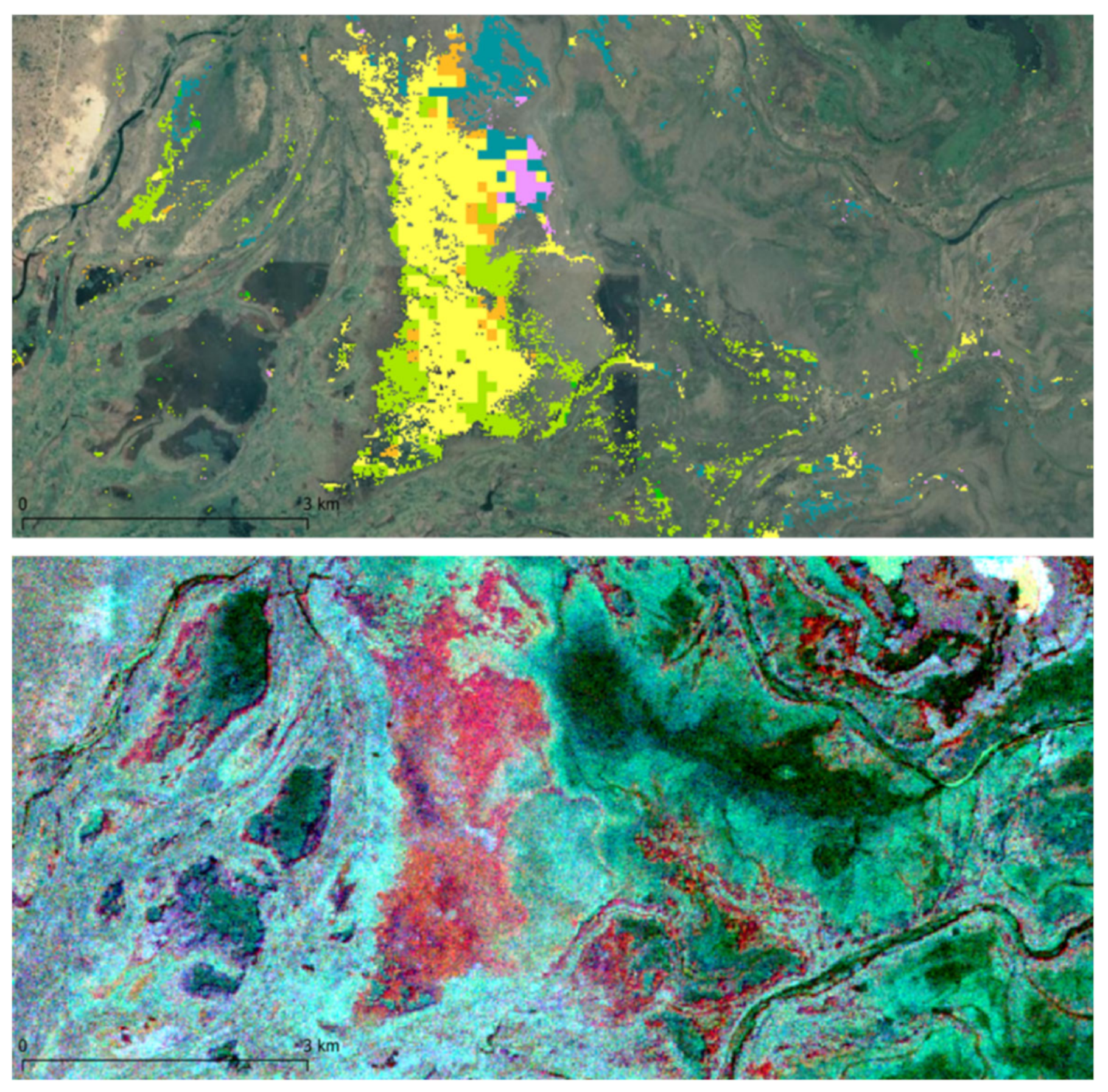
Cluster 6 pixels mostly fall within the Herbaceous Vegetation CORINE category (~54%), besides a lower percentage of the ubiquitous Deciduous Broadleaf Open Forest class (~32%) and negligible other classes (Figure 11). Its centroid corresponds to high backscatter values in C band, with an increase of almost 5 dB from ca. −8 dB to about −3 dB, while in L band backscatter stays quite constant at very low values, −19 dB in HH to −28 dB in HV polarization (Figure 10). An example of a quite compact area corresponding to this cluster is shown in Figure 15 (area c). The predominant color is in fact yellow, corresponding to Herbaceous Vegetation with smaller areas of Deciduous Broadleaf Open Forest in green. In the corresponding RGB composite change image, at the bottom of the figure, the area is mostly colored in light red, indicating in fact increase of C-band levels and no change in the other two channels. This behavior can be explained, in C band, with the double bounce interaction of thin plant stems and branches, typical of herbaceous vegetation, with underlying water, while this effect is not present in L band, due to the longer wavelength. This area appears completely dark in the S1 image acquired in January and it is classified there as “open” water. It is worth noticing that January was the peak of the flood and that the herbaceous vegetation was then likely completely submerged.
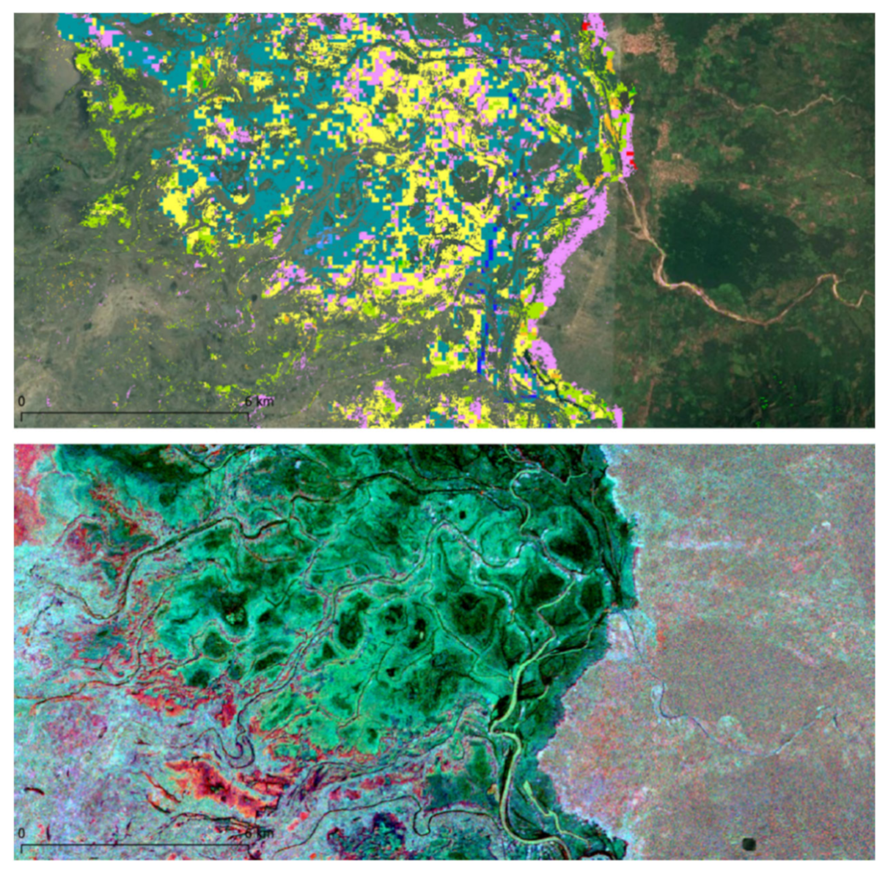
Cluster 7 falls on comparable percentages of Deciduous Broadleaf Open Forest (~22%), Herbaceous Wetland (~24%), Cropland (~20%), and Herbaceous Vegetation (~22%) (Figure 11). Its centroid exhibits a strong, −10 dB decrease in C band, while rather constant, low values in L band (Figure 10). Figure 16 shows a representative area with pixels in this cluster, as usual colored as in the CORINE color legend, showing a rather random mix of classes belonging to the above mentioned four, including a wide, compact strip of cropland (in pink), as well as large patches of wetlands (in blue/grey color). Most of the area has green color in the RGB backscatter change composite, at the bottom of the figure, with brighter shades likely corresponding to strips of vegetation along water channels, while darker tones characterize areas farther from the water courses. This in fact corresponds to strong decrease in C-band backscatter, with lower to no decrease in L-band, slightly more pronounced in HV (blue channel) than in HH (green channel) polarization. The likely interpretation of this cluster is of areas normally covered by water (such as wetlands), but which, in correspondence with the investigated event, witness an increase in water levels, overcoming the height of some short and sparse vegetation, which render the surface more specular in C band, while the effect is negligible in L band, giving almost no change in this band.
Cluster 8 has an even more variegated CORINE class composition, including Deciduous Broadleaf Open Forest (~27%), and then Herbaceous Wetland, Herbaceous Vegetation, and Cropland, each not exceeding 23% (Figure 11). This cluster seems to correspond quite precisely to areas with open water due to the flood, causing a generalized, strong backscatter decrease in both C and L band. Its position in the three plots in Figure 10 is indeed in the bottom-right quadrant, with decrease of about 10 dB in all three cases. Sample cluster areas, represented with the usual CORINE class color map in the left panel of Figure 17, correspond quite precisely with dark areas in the RGB composite on the right, indicating in fact strong generalized backscatter decrease.
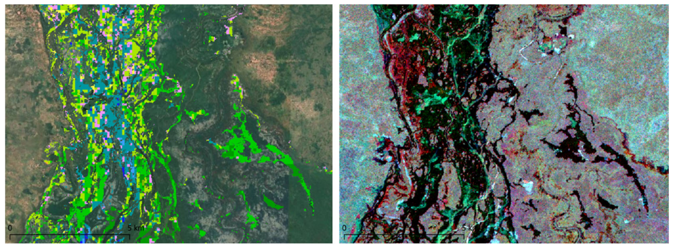
Cluster 9 covers mostly permanent water areas, which indeed form about 48% of its content as CORINE class (Figure 11). The cluster centroid is placed almost exactly on the main diagonal in all three plots in Figure 10, indicating constantly low backscatter values in all channels. Lower, but non-negligible percentages of forested classes are also covered. This can be understood by looking at Figure 18: in the left panel, we show a sample area with the cluster pixels colored in the usual CORINE color code. It can be noticed that most of the pixel correspond to the river course path, in blue color, but this is flanked by a thin strip of pixels flagged as forest (green) or cropland (pink). This non-perfect overlap of SAR derived and CORINE classes can be due to CORINE classification errors, to actual changed conditions on the ground (e.g., seasonal enlargements of the river bed), or both. An even more interesting area is the one shown in the right panel of the same figure. Here, pixels belonging to the SAR-identified permanent water cluster correspond in the CORINE map to vegetated areas, including a narrow water channel (probably too narrow to be “seen” by the coarse-resolution PROBA-V optical sensors used to produce the CORINE map), and several large ponds, equally not identified as permanent waters in the CORINE map, probably because of changed environmental conditions, among the period of PROBA-V imagery (spanning several acquisitions in the interval 2015–2018) and those of the SAR data takes (concentrated in early 2015).
Finally, we focus on cluster 12, which has a CORINE pixel composition not dissimilar from other cluster such as 5, with a high percentage of Deciduous Broadleaf Open Forest (>44%), and lower percentages of cropland and Herbaceous Vegetation (22 and 16%, respectively, Figure 11). Its centroid is roughly on the main diagonal of the C-band plot in Figure 10, while exhibiting decrease of 5–6 dB in L-band levels. Its ground cover is however heterogeneous, as its variances in all the six channels are relatively high. In fact, areas with pixels falling within this cluster may have different behaviors. We choose to show the area in Figure 19 (corresponding to window h in Figure 10), which involves a rather large patch of forest and herbaceous vegetation areas as per the CORINE map, corresponding to bright red color in the RGB composite in the bottom map. This corresponds to very strong positive change in C-band, thus standing for double-bounce increase due to water flooding of (low) vegetation, with equally strong decrease of L-band backscatter levels, thus appearing as open water at longer wavelengths. The most likely interpretation here is of a vegetation with small stems which enhance backscatter in C band, while being specular in L band. Another perhaps more likely phenomenon is the change in water levels in the two dates corresponding to C- and L-band acquisitions, with low levels in the C-band image, thus leaving vegetation sticking out from the water, while higher levels in the L-band acquisition, covering completely the short vegetation cover and causing specular reflection. This situation appears as the predominant one on the forest clearing shown on the Google imagery in the inset detail map.
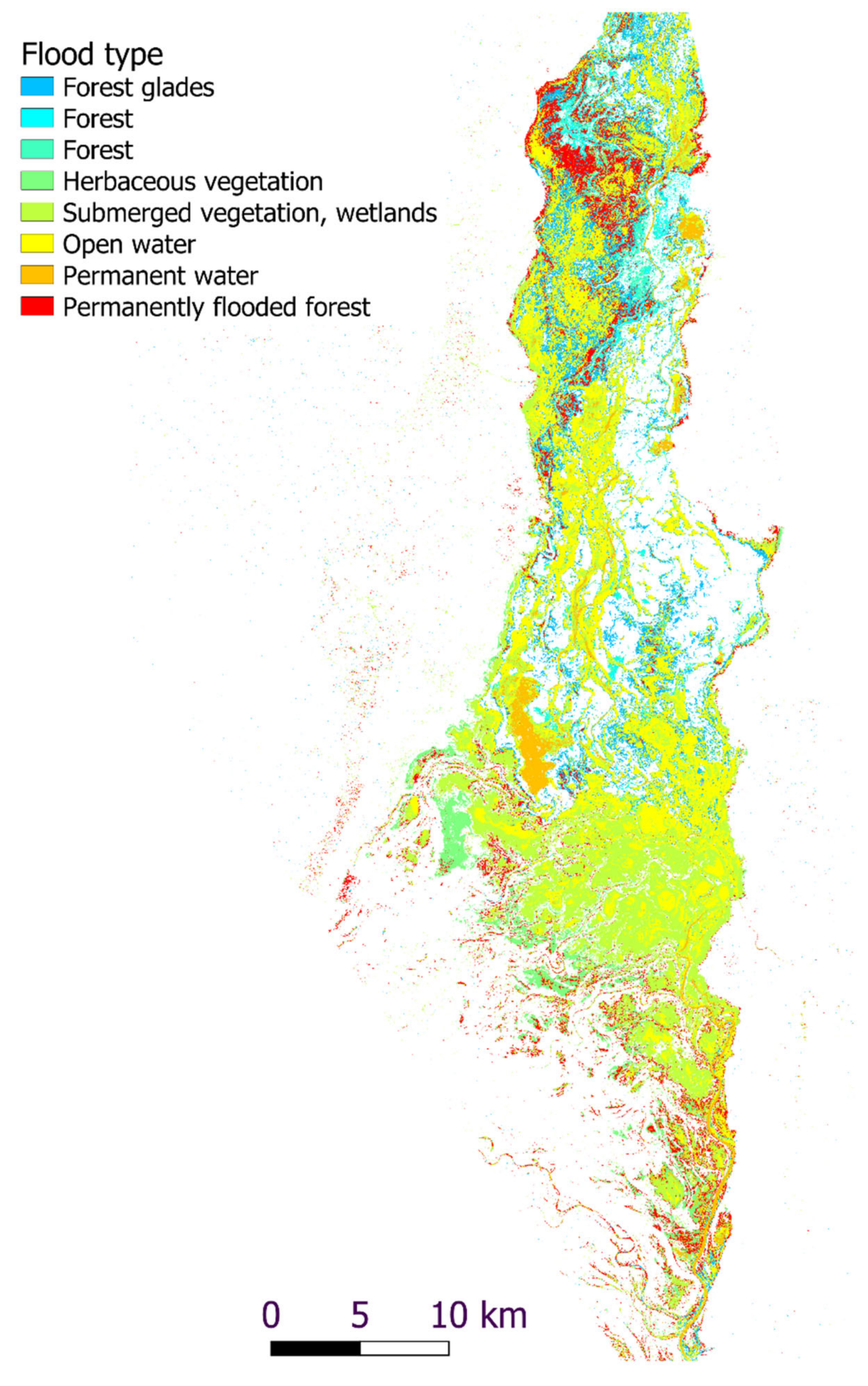
The above-described clusters can be finally cast into a map of flooded areas for the February 2015 event, highlighting the different types of microwave interaction, also according to the CORINE land cover interpretation. The map is shown in Figure 20. A heuristic mask, based on the apparent limits of the flooded areas derived from the preliminary maps of open water derived from either sensor, has been used to spatially constrain the occurrence of areas corresponding to clusters 4 and 5, which basically isolate the flooded forest stands, exhibiting strong double bounce phenomena in L-band. The map shows a rather complex texture of open water, partially and fully submerged vegetated areas, permanently flooded forests and wetlands, and forest openings at the borders of thicker stands where neither C nor L band can penetrate.
The multi-sensor map in Figure 20, together with the multi-temporal maps in Figure 2 and Figure 4, can be regarded as the main contributions of this study to the body of knowledge about remote-sensing-based flood monitoring. We remark the following final points.
Dense time series of homogeneous acquisitions from the same SAR sensor are very helpful in following the drying dynamics of a given flood event, providing information which can be exploited by hydrologists or environmental scientists to study, e.g., climate change impacts on extreme events dynamics. Currently, the only sensor able to provide such dense time series is Sentinel-1, although other missions such as the X-band Italian constellation COSMO-SkyMed are planned to increase their temporal acquisition schedule. L-band sensors such as ALOS/PALSAR 2, as shown in this work, currently do not allow more than a single co-event image for typical flood durations Multi-frequency integration is extremely useful to recognize different flooded surfaces, especially on vegetated areas, provided that simultaneous acquisitions are available. These at present are quite rare and fortuitous combinations.
Another important part of this study is land cover information, provided by the CORINE database. Although not perfectly “tuned” for these specific applications, both in terms of acquisition times and resolution, it provided invaluable insight into the nature of classes of backscattering conditions on the ground. We remark that, as for instance in the case of permanent waters, SAR-derived information could be exploited in return to update such databases.
Finally, we still remark the absence of any known independent ground truth information for this event. As underlined earlier, this is not an unusual condition for flood events, especially in less developed countries. Nevertheless, application of automated data analysis tools, together with a good deal of heuristic inference, based on indirect evidence from high-resolution optical imagery taken at various times (Google EarthTM), helped in devising convincing map products. We believe further studies should be directed to the automation of such heuristic inference, e.g., through machine learning techniques.
7. Conclusions
Flood monitoring on thickly vegetated, remote areas is important for damage assessment, as well as for studying the response and evolution of inundation phenomena in tropical countries. However, identification of water on the ground, as well as monitoring the event evolution can be challenging, due to different ground cover causing heterogenous response of the terrain surface to the presence of floodwater depending on the type of terrain and the thickness of the vegetation canopy.
In this work, we show an experiment on the integration of multi-temporal, multi-sensor, and multi-polarization SAR data with CORINE land cover information to infer consistent information about a flood phenomenon occurred in early 2015 on the African Shire River basin, in Mozambique.
We first extract information about the temporal evolution of open water flooded areas, through a K-means cluster analysis of the pixels of six Sentinel-1 images acquired at short time intervals during the event. The analysis evidenced the presence of floodwater extending over areas covered by herbaceous vegetation and cropland in the first phases of the flood, followed by a progressive shrinking of the inundated area, with final coverage of wetlands and a few forested areas. Quantification of areas affecting each of the CORINE land cover classes confirms the initial preponderance of flooded herbaceous land cover, which appears to dry faster than wetlands and forests. A similar temporal analysis performed on the two L-band images, one pre- and one co-event, highlighted significant differences in the extent and location of open water with respect to those detected in C band.
Exploiting a time interval in which no significant change is observed in the preceding temporal analysis, a multi-frequency, multi-temporal dataset including pre- and co-event imagery from Sentinel-1 (C band) and ALOS 2 (L band) sensors is then built and analyzed, again through K-means pixel clustering and comparison with CORINE land cover classes and Google imagery. The results highlight the likely presence of floodwater on different types of terrain cover, giving rise to different decrease and increase of backscatter levels in the different bands and polarizations. In particular, this allowed to determine the presence of several areas in which water is present underneath various types of vegetation causing double bounce phenomena of various intensity. A multi-sensor flood map highlighting the different interactions of floodwaters with vegetation according to the used radiation wavelengths has been finally obtained.
This kind of studies are expected to assume increasing importance as the availability of multi-frequency data from SAR satellite constellations will increase in the future. Indeed, to augment its acquisition frequency and to fill critical information gaps in the monitoring of geo-hazards at global scale by extending ground motion information to vegetated areas and by improving flood mapping, especially below vegetation, the Copernicus program is planning to include an L-band Sentinel-1-like satellite, namely ROSE-L, which is part of the six high-priority candidate missions being studied [36].
Author Contributions
All authors contributed equally to paper conceptualization, methodology setup, data analysis and validation; M.Z. and M.C.—original draft preparation; A.R. and A.D.—review and editing. All authors have read and agreed to the published version of the manuscript.
Funding
The contribution of A.R. and A.D. was supported by the Italian Ministry of Education, University and Research, in the framework of the project OT4CLIMA, D.D. 2261–6.9.2018, PON R&I 2014–2020. M. Chini contribution was supported by the Luxembourg National Research Fund through the MOSQUITO project (Grant CORE C15/SR/10380137).
Acknowledgments
The ALOS-2 PALSAR-2 data used in this study are owned by the Japan Aerospace Exploration Agency (JAXA) and were provided through the JAXA’s ALOS-2 research program (RA4, PI No. 1255).
Conflicts of Interest
The authors declare no conflict of interest.
References
- Refice, A.; D’Addabbo, A.; Capolongo, D. (Eds.) Flood Monitoring through Remote Sensing; Springer Remote Sensing/Photogrammetry; Springer International Publishing: Cham, Switzerland, 2018; ISBN 978-3-319-63958-1. [Google Scholar]
- Schumann, G.J.-P.; Bates, P.D.; Neal, J.C.; Andreadis, K.M. Measuring and Mapping Flood Processes. In Hydro-Meteorological Hazards, Risks and Disasters; Elsevier: Amsterdam, The Netherlands, 2015; pp. 35–64. ISBN 9780123964700. [Google Scholar]
- Rahman, M.S.; Di, L. A Systematic Review on Case Studies of Remote-Sensing-Based Flood Crop Loss Assessment. Agriculture 2020, 10, 131. [Google Scholar] [CrossRef] [Green Version]
- Refice, A.; Capolongo, D.; Pasquariello, G.; D’Addabbo, A.; Bovenga, F.; Nutricato, R.; Lovergine, F.P.; Pietranera, L. SAR and InSAR for Flood Monitoring: Examples with COSMO-SkyMed Data. IEEE J. Sel. Top. Appl. Earth Obs. Remote Sens. 2014, 7, 2711–2722. [Google Scholar] [CrossRef]
- Pulvirenti, L.; Pierdicca, N.; Chini, M.; Guerriero, L. Monitoring flood evolution in vegetated areas using cosmo-skymed data: The tuscany 2009 case study. IEEE J. Sel. Top. Appl. Earth Obs. Remote Sens. 2013, 6, 1807–1816. [Google Scholar] [CrossRef]
- Pierdicca, N.; Pulvirenti, L.; Chini, M.; Guerriero, L.; Candela, L. Observing floods from space: Experience gained from COSMO-SkyMed observations. Acta Astronautica 2013, 84, 122–133. [Google Scholar] [CrossRef]
- Schlaffer, S.; Matgen, P.; Hollaus, M.; Wagner, W. Flood detection from multi-temporal SAR data using harmonic analysis and change detection. Int. J. Appl. Earth Obs. Geoinf. 2015, 38, 15–24. [Google Scholar] [CrossRef]
- Capolongo, D.; Refice, A.; Bocchiola, D.; D’Addabbo, A.; Vouvalidis, K.; Soncini, A.; Zingaro, M.; Bovenga, F.; Stamatopoulos, L. Coupling multitemporal remote sensing with geomorphology and hydrological modeling for post flood recovery in the Strymonas dammed river basin (Greece). Sci. Total Environ. 2019, 651, 1958–1968. [Google Scholar] [CrossRef]
- Pulvirenti, L.; Chini, M.; Pierdicca, N.; Guerriero, L.; Ferrazzoli, P. Flood monitoring using multi-temporal COSMO-SkyMed data: Image segmentation and signature interpretation. Remote Sens. Environ. 2011, 115, 990–1002. [Google Scholar] [CrossRef]
- Chini, M.; Hostache, R.; Giustarini, L.; Matgen, P. A hierarchical split-based approach for parametric thresholding of SAR images: Flood inundation as a test case. IEEE Trans. Geosci. Remote Sens. 2017, 55, 6975–6988. [Google Scholar] [CrossRef]
- Hess, L.L.; Melack, J.M.; Simonett, D.S. Radar detection of flooding beneath the forest canopy: A review. Int. J. Remote Sens. 1990, 11, 1313–1325. [Google Scholar] [CrossRef]
- Pierdicca, N.; Pulvirenti, L.; Chini, M. Flood Mapping in Vegetated and Urban Areas and Other Challenges: Models and Methods. In Flood Monitoring through Remote Sensing; Springer: Cham, Switzerland, 2018; pp. 135–179. [Google Scholar]
- Wang, Y.; Imhoff, M.L. Simulated and observed L-HH radar backscatter from tropical mangrove forests. Int. J. Remote Sens. 1993, 14, 2819–2828. [Google Scholar] [CrossRef]
- Dabrowska-Zielinska, K.; Budzynska, M.; Tomaszewska, M.; Bartold, M.; Gatkowska, M.; Malek, I.; Turlej, K.; Napiorkowska, M. Monitoring wetlands ecosystems using ALOS PALSAR (L-Band, HV) supplemented by optical data: A case study of Biebrza Wetlands in Northeast Poland. Remote Sens. 2014, 6, 1605–1633. [Google Scholar] [CrossRef] [Green Version]
- Dabboor, M.; Brisco, B. Wetland Monitoring and Mapping Using Synthetic Aperture Radar. In Wetlands; Intech Open: London, UK, 2018; pp. 1–26. [Google Scholar]
- Manavalan, R.; Rao, Y.S.; Krishna Mohan, B. Comparative flood area analysis of C-band VH, VV, and L-band HH polarizations SAR data. Int. J. Remote Sens. 2017, 38, 4645–4654. [Google Scholar] [CrossRef]
- Pierdicca, N.; Pulvirenti, L.; Boni, G.; Squicciarino, G.; Chini, M. Mapping Flooded Vegetation Using COSMO-SkyMed: Comparison with Polarimetric and Optical Data Over Rice Fields. IEEE J. Sel. Top. Appl. Earth Obs. Remote Sens. 2017, 10, 2650–2662. [Google Scholar] [CrossRef]
- D’Addabbo, A.; Refice, A.; Pasquariello, G.; Lovergine, F.P.; Capolongo, D.; Manfreda, S. A Bayesian Network for Flood Detection Combining SAR Imagery and Ancillary Data. IEEE Trans. Geosci. Remote Sens. 2016, 54, 3612–3625. [Google Scholar] [CrossRef]
- Hong, S.-H.; Wdowinski, S. Double-Bounce Component in Cross-Polarimetric SAR From a New Scattering Target Decomposition. IEEE Trans. Geosci. Remote Sens. 2014, 52, 3039–3051. [Google Scholar] [CrossRef]
- Schlaffer, S.; Chini, M.; Dettmering, D.; Wagner, W. Mapping Wetlands in Zambia Using Seasonal Backscatter Signatures Derived from ENVISAT ASAR Time Series. Remote Sens. 2016, 8, 402. [Google Scholar] [CrossRef] [Green Version]
- Beilfuss, R.D.; dos Santos, D. Patterns of Hydrological Change in the Zambezi Delta, Mozambique; Working Paper #2 Zambezi Basin Crane and Wetland Conservation Program; International Crane Foundation: Baraboo, WI, USA, 2001. [Google Scholar]
- Nharo, T. Modeling Floods in the Middle Zambezi Basin Using Remote Sensing and Hydrological Modeling Techniques. Master’s Thesis, University of Zimbabwe, Harare, Zimbabwe, 2016. [Google Scholar]
- Singh, A. Historical Analysis of Change in Rainfall, Flow Regime and River Morphology Case Study: Zambezi Delta; UNESCO-IHE Institute for Water Education: Delft, The Netherlands, 2017. [Google Scholar]
- Beilfuss, R.D.; Moore, D.; Bento, C.; Dutton, P. Patterns of Vegetation Change in the Zambezi Delta, Mozambique; Working Paper #3 Zambezi Basin Crane and Wetland Conservation Program; International Crane Foundation: Baraboo, WI, USA, 2001. [Google Scholar]
- Davies, B.R.; Beilfuss, R.D.; Thoms, M.C. Cahora Bassa retrospective, 1974–1997: Effects of flow regulation on the Lower Zambezi River. SIL Proc. 2000, 27, 2149–2157. [Google Scholar] [CrossRef]
- Pasanisi, F.; Tebano, C.; Zarlenga, F. Indagine Morfologica su un Tratto del Fiume Zambesi, nella Repubblica del Mozambico. Misure Batimetriche ed Analisi Dei Dati; Technical Report No. RT/2015/14/ENEA; ENEA: Rome, Italy, 2015. [Google Scholar]
- Ronco, P.; Fasolato, G.; Nones, M.; Di Silvio, G. Morphological effects of damming on lower Zambezi River. Geomorphology 2010, 115, 43–55. [Google Scholar] [CrossRef]
- Shela, O. Management of shared river basins: The case of the Zambezi River. Water Policy 2000, 2, 65–81. [Google Scholar] [CrossRef]
- Lee, J.-S.; Ainsworth, T.L.; Wang, Y.; Chen, K.-S. Polarimetric SAR Speckle Filtering and the Extended Sigma Filter. IEEE Trans. Geosci. Remote Sens. 2015, 53, 1150–1160. [Google Scholar] [CrossRef]
- ESA. Land Cover CCI Product User Guide Version 2.0; ESA: Paris, France, 2017. [Google Scholar]
- Refice, A.; D’Addabbo, A.; Lovergine, F.P.; Tijani, K.; Morea, A.; Nutricato, R.; Bovenga, F.; Nitti, D.O. Monitoring Flood Extent and Area Through Multisensor, Multi-temporal Remote Sensing: The Strymonas (Greece) River Flood. In Flood Monitoring through Remote Sensing; Springer International Publishing: Cham, Switzeland, 2018; pp. 101–113. [Google Scholar]
- MacQueen, J. Some Methods for Classification and Analysis of Multivariate Observations. In Proceedings of the 5th Berkeley Symposium on Mathematical Statistics and Probability; University of California Press: Berkeley/Los Angeles, CA, USA, 1967; Volume 1, pp. 281–297. [Google Scholar]
- D’Addabbo, A.; Refice, A.; Lovergine, F.P.; Pasquariello, G. DAFNE: A Matlab toolbox for Bayesian multi-source remote sensing and ancillary data fusion, with application to flood mapping. Comput. Geosci. 2018, 112, 64–75. [Google Scholar] [CrossRef]
- Chini, M.; Chiancone, A.; Stramondo, S. Scale Object Selection (SOS) through a hierarchical segmentation by a multi-spectral per-pixel classification. Pattern Recognit. Lett. 2014, 49, 214–223. [Google Scholar] [CrossRef] [Green Version]
- Bhattacharya, A. On a measure of divergence between two multinomial populations. Indian J. Stat. 1946, 7, 401–406. [Google Scholar]
- Pierdicca, N.; Davidson, M.; Chini, M.; Dierking, W.; Djavidnia, S.; Haarpaintner, J.; Hajduch, G.; Laurin, G.V.; Lavalle, M.; López-Martínez, C.; et al. The Copernicus L-band SAR mission ROSE-L (Radar Observing System for Europe). In Active and Passive Microwave Remote Sensing for Environmental Monitoring III; Notarnicola, C., Pierdicca, N., Bovenga, F., Santi, E., Eds.; SPIE: Washington, DC, USA, 2019; Volume 11154, p. 13. [Google Scholar]
Figure 1.
(a) Location of the Zambezi River basin, (b) enlarged view with footprints of the Satellite imagery—green: Sentinel-1 (ascending and descending), cyan: ALOS 2, (2 frames); (c) detail map with locations and toponyms described in the text; (d) CORINE land cover map for the region of interest, with legend.

Figure 2.
Left: multi-temporal flood map for an area of the Shire basin, obtained by Sentinel-1 images. Areas with darker colors are flooded for longer periods, thus depicting the shrinking of the flooded surface from the first (22 January 2015), up to the last flood date (27 February 2015) reported in the legend. Darkest areas are covered by permanent water (at the post-event date of 22 April 2015). Right: maps of flooded areas on each of the 6 S1 acquisition dates, with colors corresponding to the CORINE land cover classes (shown in Figure 1).

Figure 3.
Estimation of the areas flooded for each CORINE land cover class, in the sequence of Sentinel-1 images. Colors in the legend follow the standard CORINE class labels shown in Figure 1.
Figure 3.
Estimation of the areas flooded for each CORINE land cover class, in the sequence of Sentinel-1 images. Colors in the legend follow the standard CORINE class labels shown in Figure 1.

Figure 4.
Left: multi-temporal open-water flood map for the Shire basin, obtained by ALOS-2 images. Areas with darker colors are flooded for longer periods, thus depicting the evolution of the flooded surface from the first, pre-event to the second, co-event image, as reported in the legend. Right: maps of flooded areas on each of the 2 A2 acquisition dates, with colors corresponding to the CORINE land cover classes (shown in Figure 1).

Figure 5.
Estimation of the areas flooded for each CORINE land cover class, in the sequence of Sentinel-1 images. Colors in the legend follow the standard CORINE class labels.
Figure 5.
Estimation of the areas flooded for each CORINE land cover class, in the sequence of Sentinel-1 images. Colors in the legend follow the standard CORINE class labels.

Figure 6.
(a) RGB combination of the two S1 images acquired on 3 (red) and 15 (green and blue channels) February 2015. (b) RGB combination of the A2 images acquired on 1 December 2014 (red) and 9 February 2015 (green and blue channels).
Figure 6.
(a) RGB combination of the two S1 images acquired on 3 (red) and 15 (green and blue channels) February 2015. (b) RGB combination of the A2 images acquired on 1 December 2014 (red) and 9 February 2015 (green and blue channels).

Figure 7.
Histograms of synthetic aperture radar (SAR) intensities over the CORINE land cover classes found on the image, for (a) C band, (b) L band.
Figure 7.
Histograms of synthetic aperture radar (SAR) intensities over the CORINE land cover classes found on the image, for (a) C band, (b) L band.

Figure 8.
Left: K-means cluster map obtained with K = 21 clusters. Right: the three scatterplots show the cluster centers in the 3 planes whose axes are the 3 channels backscatter values in the pre- and flood acquisition dates. Cluster numbers are reported next to each colored dot to facilitate recognition in the legend and thus in the map.

Figure 9.
Minimum Bhattacharyya distance as a function of the number of clusters in the multi-frequency dataset.
Figure 9.
Minimum Bhattacharyya distance as a function of the number of clusters in the multi-frequency dataset.

Figure 10.
As in Figure 8, with K = 12 clusters. White rectangles on the left map, labeled from a to h, highlight detail areas shown enlarged in the subsequent figures.
Figure 10.
As in Figure 8, with K = 12 clusters. White rectangles on the left map, labeled from a to h, highlight detail areas shown enlarged in the subsequent figures.

Figure 11.
Class pixel relative populations for the multi-temporal K-means classified image.

Figure 12.
Multifrequency RGB (red-green-blue) intensity ratio combination: red—S1-VV change, green—A2-HH change, blue—A2-HV change. Input values are saturated at ±10 dB, as illustrated by the inset color cube.
Figure 12.
Multifrequency RGB (red-green-blue) intensity ratio combination: red—S1-VV change, green—A2-HH change, blue—A2-HV change. Input values are saturated at ±10 dB, as illustrated by the inset color cube.

Figure 13.
Detail area (a) in Figure 10. Left: pixels corresponding to cluster 3, colored according to the underlying CORINE class; inset shows a particular area corresponding to a forest glade; background from Google EarthTM imagery. Right: same area, extracted from the RGB change image in Figure 12.

Figure 14.
Detail area (b) in Figure 10. Top: pixels corresponding to clusters 4 and 5, colored according to the underlying CORINE class; inset shows a detail area (see text for explanation); background from Google EarthTM imagery. Bottom: same area, extracted from the RGB change image in Figure 12.

Figure 15.
Detail area (c) in Figure 10. Top: pixels corresponding to cluster 6, colored according to the underlying CORINE class; background from Google EarthTM imagery. Bottom: same area, extracted from the RGB change image in Figure 12.

Figure 16.
Detail area (d) in Figure 10. Top: pixels corresponding to cluster 7, colored according to the underlying CORINE class; background from Google Earth™ imagery. Bottom: same area, extracted from the RGB change image in Figure 12.

Figure 17.
Detail area (e) in Figure 10. Left: pixels corresponding to cluster 8, colored according to the underlying CORINE class; background from Google Earth™ imagery. Right: same area, extracted from the RGB change image in Figure 12.

Figure 18.
Left: Detail area (f) in Figure 10. Right: Detail area (g) in Figure 10. Pixels corresponding to cluster 9 are colored according to the underlying CORINE class; background from Google EarthTM imagery.

Figure 19.
Detail area (h) in Figure 10. Top: pixels corresponding to cluster 12, colored according to the underlying CORINE class; background from Google EarthTM imagery. Bottom: same area, extracted from the RGB change image in Figure 12. Inset shows a forest clearing corresponding to the reddish area in the SAR change color composite.

Figure 20.
Flood map resulting from the integration of the multi-frequency information. Legend reports the interpretation of the cluster typologies, colored according to the scheme as in Figure 10.
Figure 20.
Flood map resulting from the integration of the multi-frequency information. Legend reports the interpretation of the cluster typologies, colored according to the scheme as in Figure 10.


Table 1.
Details on the used imagery. A = ascending, D = descending geometry. Images indicated in red bold text color are those selected for the subsequent multi-frequency analysis.
Table 1.
Details on the used imagery. A = ascending, D = descending geometry. Images indicated in red bold text color are those selected for the subsequent multi-frequency analysis.
| Sensor | Date | Polarization | Geometry |
|---|---|---|---|
| ALOS 2 | 1 December 2014 | HH, HV | A |
| Sentinel-1 | 29 December 2014 | VV | D |
| Sentinel-1 | 22 January 2015 | VV | D |
| Sentinel-1 | 3 February 2015 | VV | D |
| ALOS 2 | 9 February 2015 | HH, HV | A |
| Sentinel-1 | 15 February 2015 | VV | D |
| Sentinel-1 | 21 February 2015 | VV | A |
| Sentinel-1 | 27 February 2015 | VV | D |
| Sentinel-1 | 22 April 2015 | VV | A |
© 2020 by the authors. Licensee MDPI, Basel, Switzerland. This article is an open access article distributed under the terms and conditions of the Creative Commons Attribution (CC BY) license (http://creativecommons.org/licenses/by/4.0/).
Share and Cite
MDPI and ACS Style
Refice, A.; Zingaro, M.; D’Addabbo, A.; Chini, M. Integrating C- and L-Band SAR Imagery for Detailed Flood Monitoring of Remote Vegetated Areas. Water 2020, 12, 2745. https://doi.org/10.3390/w12102745
AMA Style
Refice A, Zingaro M, D’Addabbo A, Chini M. Integrating C- and L-Band SAR Imagery for Detailed Flood Monitoring of Remote Vegetated Areas. Water. 2020; 12(10):2745. https://doi.org/10.3390/w12102745
Chicago/Turabian StyleRefice, Alberto, Marina Zingaro, Annarita D’Addabbo, and Marco Chini. 2020. "Integrating C- and L-Band SAR Imagery for Detailed Flood Monitoring of Remote Vegetated Areas" Water 12, no. 10: 2745. https://doi.org/10.3390/w12102745
Note that from the first issue of 2016, this journal uses article numbers instead of page numbers. See further details here.