Flood Hazard Assessment in Data-Scarce Watersheds Using Model Coupling, Event Sampling, and Survey Data
by
 , , and
Jorge Hurtado-Pidal
1,* ,
,
Juan S. Acero Triana
2,
Edgar Espitia-Sarmiento
3 and
Fernando Jarrín-Pérez
4 1
Department of Territorial Planning, Faculty of Environmental Sciences and EULA-Centre, Universidad de Concepción, 4070386 Concepción, Chile
2
Department of Agricultural and Biological Engineering, University of Illinois, 1304 West Pennsylvania Avenue, Urbana, IL 61801, USA
3
Water and Aquatic Resources Research Group (GIRHA), Universidad Regional Amazónica Ikiam, 150101 Tena, Ecuador
4
Department of Biological & Agricultural Engineering, Texas A&M University, TX 77843, USA
*
Author to whom correspondence should be addressed.
Water 2020, 12(10), 2768; https://doi.org/10.3390/w12102768
Submission received: 8 July 2020
/
Revised: 24 September 2020
/
Accepted: 1 October 2020
/
Published: 4 October 2020
(This article belongs to the Special Issue Advances in Flash Flood Forecasting)
Abstract
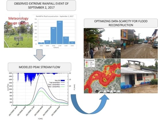
:The application of hydrologic and hydrodynamic models in flash flood hazard assessment is mainly limited by the availability of robust monitoring systems and long-term hydro-meteorological observations. Nevertheless, several studies have demonstrated that coupled modeling approaches based on event sampling (short-term observations) may cope with the lack of observed input data. This study evaluated the use of storm events and flood-survey reports to develop and validate a modeling framework for flash flood hazard assessment in data-scarce watersheds. Specifically, we coupled the hydrologic modeling system (HEC-HMS) and the Nays2Dflood hydrodynamic solver to simulate the system response to several storm events including one, equivalent in magnitude to a 500-year event, that flooded the City of Tena (Ecuador) on 2 September, 2017. Results from the coupled approach showed satisfactory model performance in simulating streamflow and water depths (0.40 ≤ Nash-Sutcliffe coefficient ≤ 0.95; −3.67% ≤ Percent Bias ≤ 23.4%) in six of the eight evaluated events, and a good agreement between simulated and surveyed flooded areas (Fit Index = 0.8) after the 500-year storm. The proposed methodology can be used by modelers and decision-makers for flood impact assessment in data-scarce watersheds and as a starting point for the establishment of flood forecasting systems to lessen the impacts of flood events at the local scale.
1. Introduction
The assessment of natural hazards, such as flash floods, remains a challenging issue in environmental sciences [1]. Flash floods caused by extreme rainfall events associated with climate change have increased in the past few years [2,3,4]. Thus, the development and implementation of measures that diminish flash flood impacts and safeguard people and civil infrastructure are imperative. In this context, numerical models have been found to be reliable tools for flash flood hazard assessment. Specifically, hydrological and hydrodynamic models have been widely applied to describe flash flood dynamics at the watershed scale and project potential impacts on urban areas. Hydrological models (e.g., HEC-HMS, SWAT, MIKE 11, HBV, Top Model) have been widely used to simulate precipitation-runoff processes due to the ease of their implementation [1]. Although these models can accurately estimate streamflow patterns across complex watersheds, they do not provide a comprehensive representation of water flow in riverbanks and floodplains. On the other hand, hydrodynamic models (e.g., MIKE 21, LISFLOOD-FP, DELFT-2D, IBER, Nays2DFlood), which are based on more complex formulations, can represent streamflow data in terms of water depths and flow velocities across river channels and floodplains [5,6,7,8,9] but with a larger expense in computational and data resources [10,11]. External coupling approaches that combine hydrological and hydrodynamic models have shown satisfactory performance in representing flood extents while requiring a reduced computational burden and data [12,13,14,15,16]. The information generated by combining these models may be used to reconstruct historical flood events or evaluate the plausible response of the hydrologic system to present or future stressors (e.g., climate and land-use changes) [17]. Given that hydrologic and hydrodynamic models play a crucial role in the design of flooding control structures, flood risk management, and mitigation policy-making, they need to be tested from a strict scientific point of view [18,19,20,21,22]. Model reliability depends on two key factors, namely, the model formulation that describes the system and the input data used to set up the model [11,23,24,25,26].
In developing countries, the availability and quality of hydrometeorological data represent a significant constraint for the implementation of hydrological and hydrodynamic models due to the absence of robust monitoring networks and the lack of long-term hydro-meteorological observations [27]. The scarcity of reliable input data hinders the models’ ability to represent the hydrological dynamics. Consequently, the application of hydrological and hydrodynamic models in data-scarce environments is prone to equifinality (i.e., to generate a similar systemic response under distinct model parameterizations) and high uncertainty, even after a successful calibration/validation process [28]. In other terms, modeling outputs under data scarcity conditions may not enhance the basic understanding of the processes taking place in the hydrologic system and appropriately represent the watershed’s natural characteristics [29].
In the absence of long-term observations, event sampling data may provide sufficient information to perform hydrological and hydrodynamic simulations. In this sense, several studies have found that the degree of hydrological information obtained by processing data from several storm events is comparable to that obtained by processing long-term data series [30,31,32,33,34,35,36]. The implementation of externally coupled models with event sampling data for flood hazard assessment may be quite relevant in zones with high spatial precipitation variability such as those located in the Andes-Amazon transition [37], where monitoring networks are sparse and recently established.
This study evaluated the potential use of event sampling and survey data for flash flood hazard assessment in data-scarce watersheds. Specifically, this study was geared to (1) implement a coupled framework to simulate in-stream flow and flow velocity and water depths across floodplains against short precipitation-runoff events in the data-scarce Tena River Watershed in Ecuador, and (2) evaluate the ability of the modeling framework to recreate the flood intensity due to a 500-year precipitation event that flooded the city of Tena on 2 September, 2017. Despite the fact that this city, like many others in the Amazon Basin, has experienced several flood events during recent years (2008, 2010, 2016, 2017) that have caused fatalities and significant economic losses [38,39], no flood management system has been implemented. The methodology and findings from this study may be used in similar watersheds with scarce data and for the establishment of flood forecasting systems.
2. Materials and Methods
2.1. Study Area
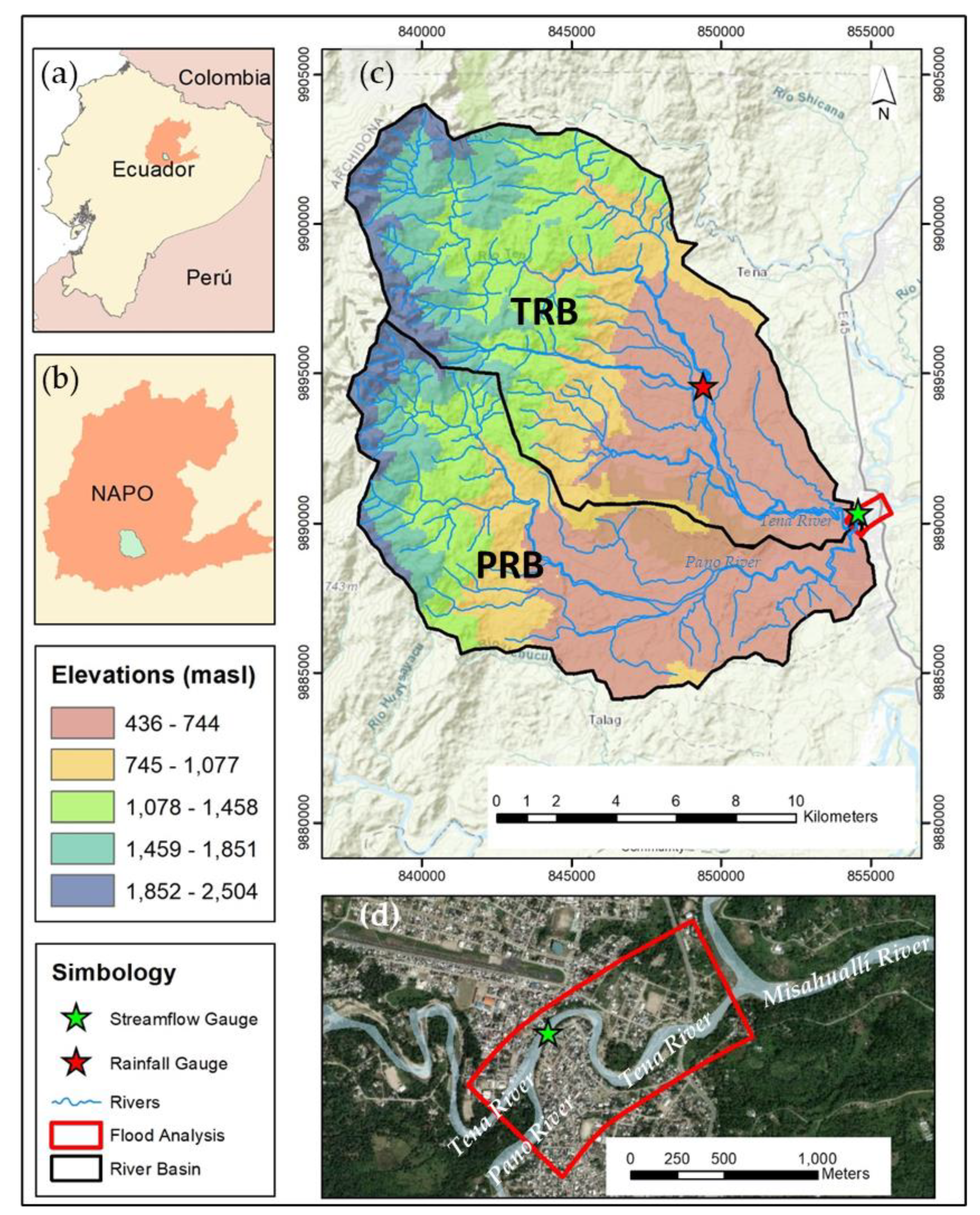
The study area comprises the Tena River Basin (TRB) and the Pano River Basin (PRB), which converge on the city of Tena (Napo province, Ecuador) and cover a drainage area of 235 km2 (Figure 1). The basins depict a very steep relief with a terrain elevation ranging from 500 to 2500 m above mean sea level (mamsl; Figure 1c) and an average slope of approximately 22.4%. The main stem of each river extends for 28 and 25 km for TRB and PRB, respectively, with a mean slope of 7%. The domain for the flood hazard assessment in the city of Tena considered a river segment of 1.7 km (Figure 1d) that has a mean slope of 0.03%. Its width and bankfull area are equal to 50 m and 362 m2, respectively, and its bed is composed of coarse material such as gravels (~5 cm) and cobbles (~25 cm). TRB and PRB have similar characteristics in terms of their geology, morphology, soil composition, land use, and climate. Both basins are part of a tertiary cretaceous sedimentary basin with predominant alluvial deposits. The soils, classified as hydrated Andisols formed in volcanic ash, that are predominantly sandy clay and sandy loam in the upper and lower parts of the watershed, respectively [40], remain saturated most of the time. This is explained by the low evapotranspiration rates of the cloud forest located in the upper part of the watershed [41], which, together with shrubs and herbaceous plants, cover 65% of the area. The lower part, on the other hand, is covered by secondary forest, pasture, and crops such as corn, cacao, and cassava (35%) [42].
In accordance with the Köppen climate classification, the study area can be defined as tropical rainforest (Af), i.e., the climate is strongly influenced by humid air masses coming from the remaining portion of the vast Amazon Basin in the east [43]. The mean annual precipitation in the city of Tena is estimated at 3500 mm, while in the upper zone of the study area, it could exceed 4000 mm. The mean annual temperature is approximately 25 °C [38].
The city has experienced a disorderly urban growth in recent decades that has occupied areas susceptible to flooding (low terraces), where nowadays approximately 3000 people live [44]. Several climate scenarios for this region have projected a progressive increase in the occurrence of extreme precipitation events until the end of the century [45,46,47,48], which may imply a higher flood risk.
2.2. Data
Soil characteristics and land cover data for the TRB and PRB were derived from thematic maps of the SIGTIERRAS project (STP), available at the spatial scale of 1:25,000 [42]. The watershed morphological parameters for the hydrological modeling (Table 1) were derived from a 30-m digital elevation model (DEM) produced by the SRTM (Shuttle Radar Topographic Mission) [49], while the topography of the river segment and floodplains for the hydrodynamic modeling were derived from a 5-m DEM surveyed by the STP through Aerial Photogrammetry. In the latter, the topography of the main channel was adjusted with ground control points, and false elevation values were corrected [42]. It is important to note that the DEM described the terrain elevation, and consequently, it did not represent objects and obstacles such as buildings.
Hydrometeorological monitoring initiatives in the watershed started in 2013 with the foundation of the Ikiam University, which installed an automatic weather station and an automatic radar streamflow gauge [50] in 2015 and 2018, respectively (Figure 1). These gauges record precipitation, streamflow, water depth, and flow velocity patterns using a one-minute time step. The data is available at http://meteorologia.ikiam.edu.ec:3838/meteoviewer/. The streamflow gauging station is a SOMMER RQ-30, which comprises a radar sensor for water level and flow velocity measurement [50]. The cross-section area (A) is computed as a function of the water level, and then used to calculate the streamflow (Q = A × V × k; k = correction factor). A discharge table is generated from the cross-section areas and the k-factors as a function of the water level corrected by a reference measurement. The cross section of the channel at the measuring point was determined with a detailed topographic survey.
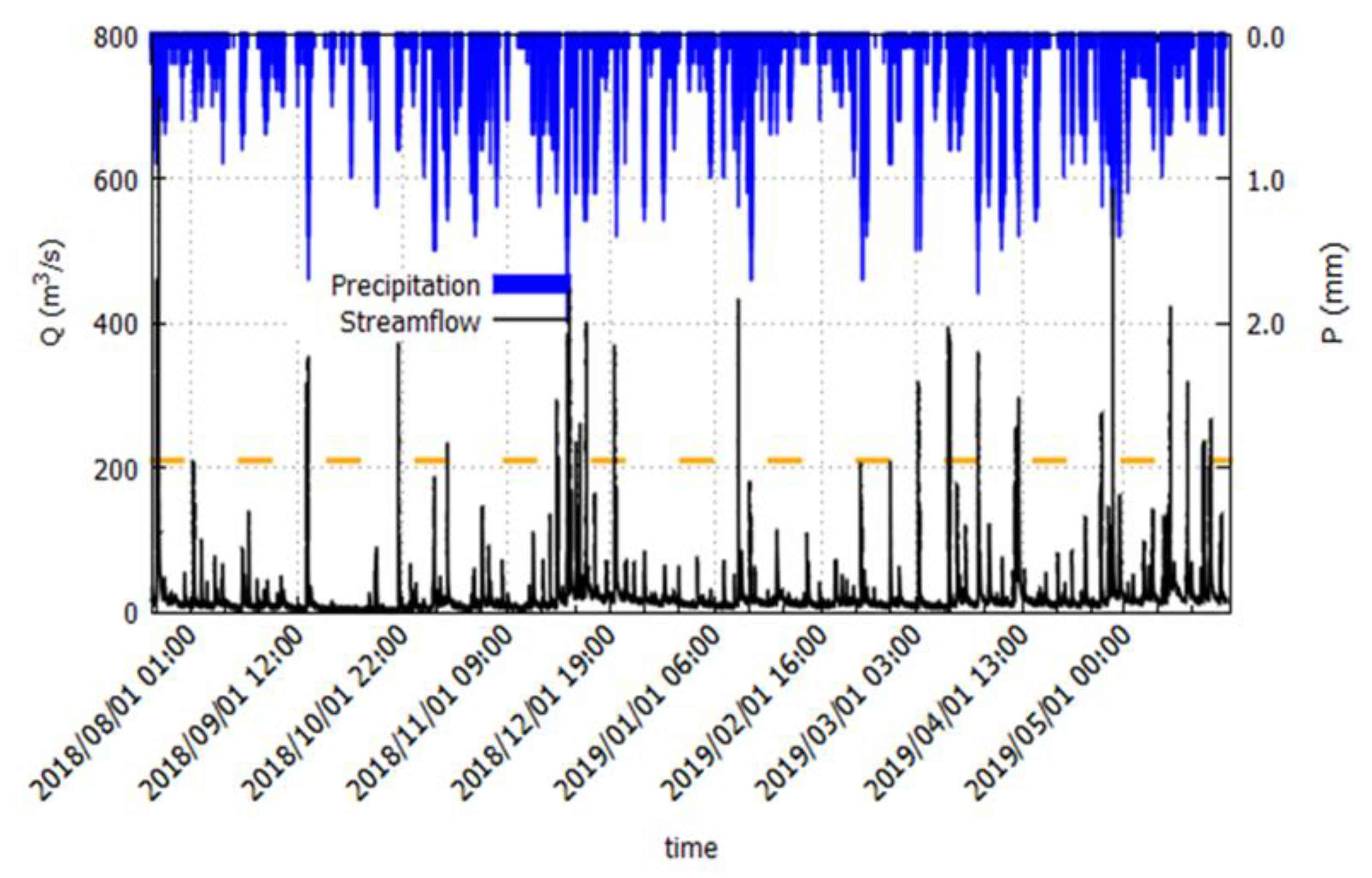
Given that this study focuses on flash flood hazard assessment, for the calibration and validation of the modeling framework, we only considered storm events that have generated a significant streamflow. These were events that generated a streamflow over 211 m3/s. This streamflow threshold was defined following the methodology proposed by Reynolds et al. [30], using the annual minimum from monthly maximum records instead of the annual mean. This obeyed the short time-series available for the streamflow (1 year; Figure 2). As a result, eight events were selected for the period between July 2018 and May 2019 (Table 2). E1 and E8 were the storm events with the longest durations (48 h), while E3 the event with the shortest (20 h) (Table 2). Likewise, the maximum and minimum peak flows were recorded for E1 (714.2 m3/s) and E3 (234.8 m3/s), respectively (Table 2).
In September 2017, an extreme precipitation event flooded the city of Tena. It had a duration of 13 h with a 1.25-h period that registered a maximum intensity of 120 mm/h. In accordance with a study of heavy precipitation events in Ecuador developed by the National Hydrometeorological Institute (INAMHI) [51], the characteristics of the 2017 extreme event were equivalent to those of an event with a 500-year return period. This INAMHI study used a meteorological station located 10 km to the northeast of our study area and with more than 50 years of records to determine the characteristics of precipitation events with different return periods. Among them, a 500-year event was described as that with a maximum intensity of 120 mm/h for a period of at least 1.25 h. In order to reproduce the flooding generated by the 2017 event and evaluate whether it may serve as a starting point for the establishment of a regional flood forecasting system, we employed our modeling framework to cope with the lack of streamflow records for the period when this 500-year event took place.
2.3. Hydrological Modeling
We set up a lumped HEC-HMS model (4.2.1 version) [52] to simulate streamflow in the main stem of PRB and TRB using the curve number (CN) and the synthetic unit hydrograph methods, both of which were developed by the Soil Conservation Service (SCS; now NRCS) [53,54,55]. The resulting hydrographs for PRB and TRB were combined without implementing any routing technique at the junction of the rivers in the city of Tena (Figure 1d). The CN is defined in terms of land cover, soil type, and antecedent soil moisture conditions. The latter is a crucial parameter that may reduce or increase the soil infiltration capacity [56], and hence, affect the amount of runoff. Initial values of CN, time of concentration (tc), and lag time (lag) were derived from previous studies performed in the study area, DEM processing, and the analysis of precipitation and streamflow time series, and then adjusted during calibration. According to Fernandez et al. [57], CN values of 90 for PRB and 87 for TRB (Table 1) accurately represent the soil saturated and the high surface runoff conditions in the basins. The tc, representing the hypothetical time that water would require to reach the watershed outlet from the remotest point [54], was expressed in terms of the river channel length and the elevation difference between the highest and lowest points of each basin using the Kirpich’s equation [58]. The lag, which corresponds to the delay or time difference between the peak precipitation and peak streamflow, was calculated as 60% of tc [52]. The initial lag values for PRB and TRB were equal to 108 and 114 min, respectively. All the initial hydrological parameters used in this study are shown in Table 1.
The built-in automatic parameter estimation algorithm within the HEC-HMS interface [59] was employed for model calibration, where the model was calibrated for event E1 and validated for events E2-8. The goodness-of-fit of the model was evaluated by comparing the observed and simulated streamflow using the Nash-Sutcliffe efficiency coefficient (NSE) and the Percent Bias (PBIAS). The NSE indicates how well the observed and simulated data fit a 1:1 line [60], while the PBIAS measures the average tendency of the simulated data to underestimate or overestimate the streamflow compared to the observations [22]. The model parameters were adjusted until the model reached a ‘very good’ performance in accordance with the Moriasi et al. [21] ratings, where the model performance metrics were computed considering all values at one-minute time steps over the event duration (Table 2).
2.4. Hydrodynamic Modeling
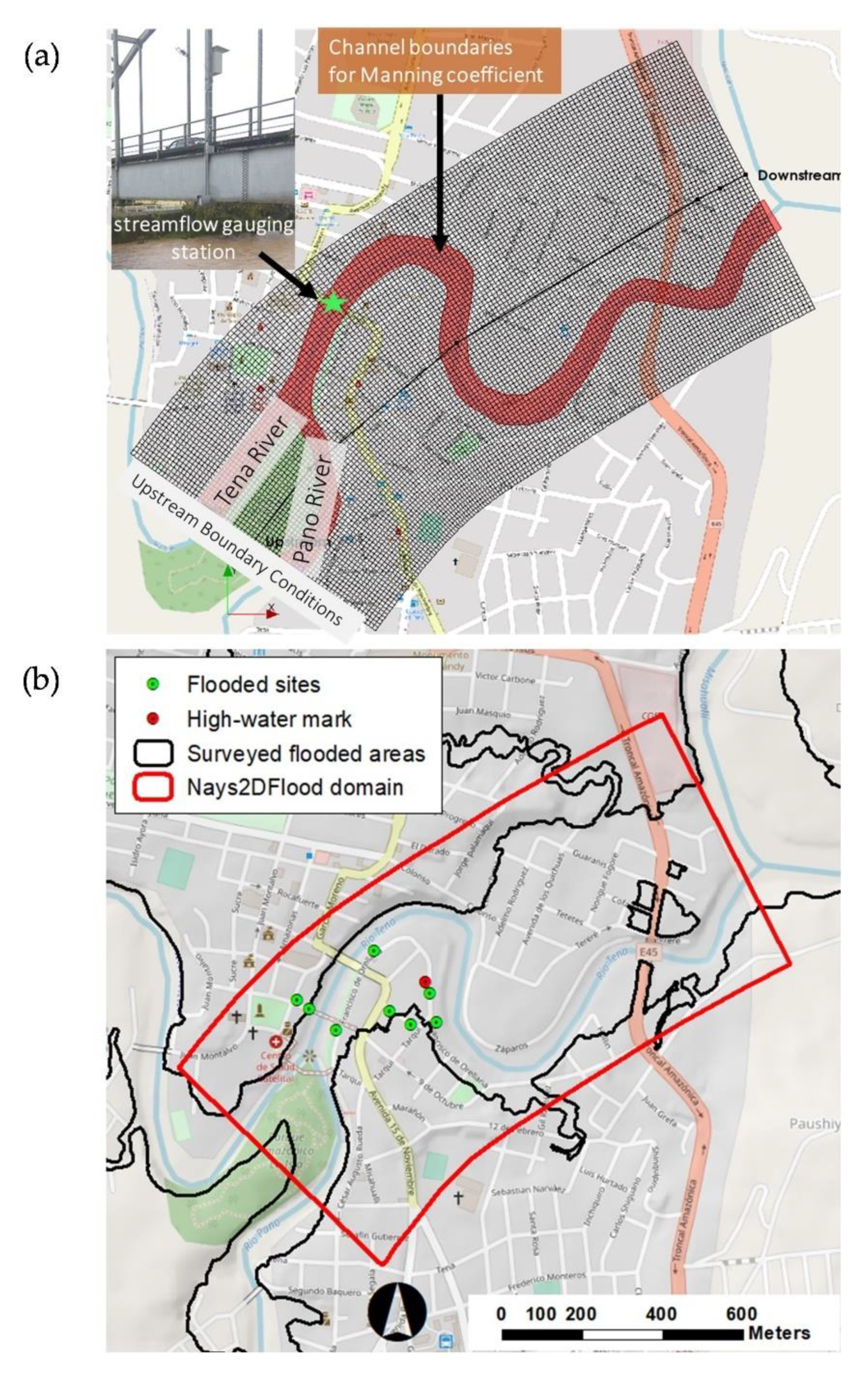
Nays2DFlood solver (3.0.0 version) [8] was used for hydrodynamic modeling. Nays2DFlood is an open-source flood flow solver for two-dimensional unsteady flow problems. It implements the continuity and momentum equations in a curvilinear coordinate system where water depths and flow velocities are the main model outputs [61,62]. For the domain used for flood hazard assessment in the city of Tena, we employed a 1-km2 structured grid that comprises 10,000 × 10-m square cells (Figure 3). This simulation area encompassed the overflown section of the main channel and the urban areas that are more prone to flooding. The upstream boundary conditions were defined using the hydrographs generated by the hydrologic model for the Tena and Pano rivers (Figure 3a) while the downstream boundary conditions, located before the confluence of the Tena and Misahuallí rivers (Figure 1), were set as free outflow. Free outflow means the simulation results for the grid cells adjacent to the boundary grid cells are given to the boundary grid cells as their boundary condition [8]. Specifically, the initial water depth was set to 0.5 m, which corresponds to the water depth at the baseflow. Additionally, model calculations were performed using a time step of 0.05 s with the model outputs being printed every 60 s.
The cell roughness characteristics were estimated by comparing aerial photographs and land cover data with tabulated roughness values. Among all the parameters, the Manning’s coefficient (n) is one of the most important for hydrodynamic modeling [11]. It represents the average flow resistance in the water profile [8]. We used an initial n value of 0.025 (natural channels with no vegetation) for the main channel [63]. For the floodplains, an equivalent Manning coefficient was implemented resembling the roughness of pavement and other urban areas (n = 0.05) [64]. Given that Nays2DFlood employs an implicit finite difference scheme to solve the advection equation, during the simulation, the water flow variables need to be spatially interpolated at each time step. Specifically, this study used the constrained interpolation profile (CIP), which is a high-order, accurate method that fits a third-order polynomial to reduce numerical diffusion. One of the CIP advantages is that a small number of adjacent cells is required to obtain an accurate estimation of the advection terms [12].
There are several techniques for the calibration and validation of hydrodynamic models based on single or multiple data sources such as remote sensing, survey data, and historical records [65,66,67,68,69]. In this study, the coefficient of Manning was manually adjusted until the error between the observed and simulated water depths and flow velocities was the minimum possible at the radar streamflow gauge located in the main channel (Figure 1). It is important to note that during flash flood events, the kinematic wave (gravitational forces) prevails over the dynamic wave (inertial forces). Therefore, the use of flow velocities and water depths is suitable for calibrating the Manning’s coefficient for the main channel, where the flow is predominantly one-dimensional [70,71]. The calibration and validation of the Manning’s coefficient of the river reach took into account the six storm events that were calibrated and validated for the hydrologic model (i.e., E1-E3, E5, E6, and E8) and one that occurred in 2017. Events E4 and E7 were not considered because of the unsatisfactory performance of HEC-HMS in simulating their streamflow patterns (Figure 4). The same model metrics (NSE and PBIAS) used for the hydrological modeling were used to evaluate the performance of Nays2DFlood.
In addition to the water depths and flow velocities at the gauging station, we used a polygon of flooded areas, additional control points of flooded sites, and a high-water mark (Figure 3b) to validate the performance of the model in simulating the 2017 extreme event. The flooded areas generated by the hydrodynamic model were evaluated using the fit index (better known as F index) [65,72], which measures the degree of overlap between the observed and simulated flooded areas from 0 to 1, where F = 1 represents a perfect overlap, and F = 0 represents no overlap. The F index is computed by dividing the spatial intersection between the observed and simulated flood areas by their spatial union.
2.5. Flood Hazard Mapping
The most relevant physical characteristics of flood events are flow velocity, water depth, and duration, which may determine their intensity and destructive capacity, and hence, may provide a measure of its hazard [73,74]. We built flood intensity maps for the 2017 flood event, postprocessing the results from the hydrodynamic simulations in GIS tools and using the flood intensity categories proposed by Cançado et al. [75] (Table 3). The flood hazard mapping was only implemented for the 2017 event because, within the available precipitation records, this flood event had survey data (flooded areas and points) which was useful for validation.
3. Results and Discussion
3.1. HEC-HMS Calibration
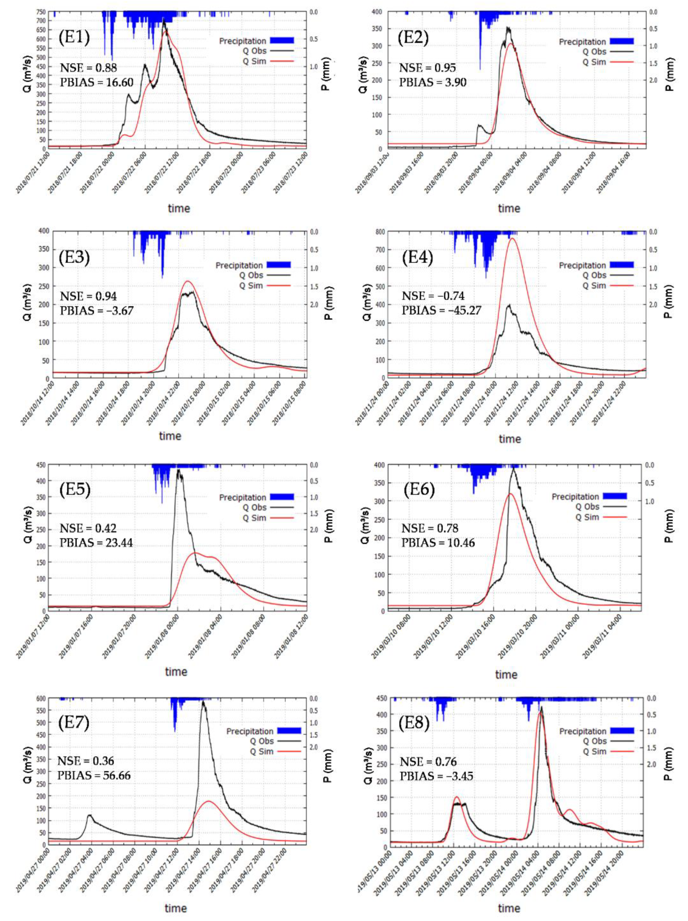
The performance of HEC-HMS in simulating the streamflow at one-minute time steps showed satisfactory results (Table 4 and Figure 4). In accordance with the Moriasi et al. [21] guidelines for calibrating hydrologic models, the NSE (0.88) and PBIAS (16.6%) for the calibration event (E1; Figure 4) indicated a good fit between the observed and simulated streamflow. Similarly, in four (E2, E3, E6, E8) of the seven validation events, the hydrologic model had a satisfactory performance (0.76 ≤ NSE ≤ 0.95; −3.67% ≤ PBIAS ≤ 10.46%; Figure 4). Since high performance metrics are difficult to achieve using a one-minute time step, and the Moriasi et al. [21] performance ratings are for monthly time-step evaluations, we considered that our model had also an acceptable performance in simulating event E5, which obtained a NSE of 0.42 and a PBIAS of 23.44% (Figure 4).
This was supported by other studies [76,77] that have stated that simulations with a daily (or smaller time steps) NSE as low as 0.4 may be considered acceptable. Consequently, five of the seven validation events had satisfactory results. Despite the fact that the performance of the model was not validated in two events (E4 and E7; Figure 4), our modeling framework was reliable in 71.4% (75% if considering the calibration event as well) of the cases, making it suitable for flood modeling. The low performance in the aforementioned two events may be explained by the spatial variability of the precipitation across the study area, which could not be fully described by the single weather station available for this study. Recall that precipitation is not monitored in PRB; this may explain some of the differences between the observed and simulated streamflow. Despite these limitations, the results were promising, taking into account the data-scarce condition of the study area and the fact that nowadays, flood prediction systems have not been deployed by the local authorities. The time difference between the observed and simulated peak flow ranged from −27 minutes to 87 minutes, with a mean value of 15 minutes, where the highest error was observed for E5 (Table 4).
The latter may imply some limitations for flood progress monitoring and forecasting, and a late response to such events from the local authorities. We believe that the modeling errors were related to the difficulty of describing the spatio-temporal patterns of every precipitation event that occurred across PRB and TRB due to the lack of multiple monitoring points. However, the results showed that in most of the cases, the single precipitation gauge available in the study area was able to provide sufficient information for simulating the streamflow in the Tena River. More efforts should be made to improve the monitoring system in the study area.
The adjusted CN values for PRB and TRB were 84 and 81, respectively, being very close to the initial assumption. The optimum lag time values, on the other hand, were 125 minutes for PRB and 130 minutes for TRB, approximately 15% greater than the initial values. Similar results for the lag time were obtained in previous studies based on morphometric analyses [57]. The high CN and low lag values indicated a fast watershed response to precipitation. This was explained by the combined effect of intense precipitation patterns, steep slopes, and high water storage capacity of clay and loam soil types. Recall that soils are saturated most of the time due to the humid environment and the cloud forest in the upper part of the study area, which has low evapotranspiration rates and allows the soil to remain moist [41]. Moreover, steep hillslopes in the upper zones of PRB and TRB facilitate surface runoff [78,79]. Under these conditions, surface runoff may be generated by both infiltration and saturation excess [80,81,82]. It is important to note that although TRB and PRB are densely forested, the ability of this cover to attenuate floods is limited [83,84].
3.2. Nays2DFlood Calibration and Reconstruction of the 500-Year Flood Event
The Manning coefficient for the channel and the floodplains was simultaneously calibrated and validated. As a result, a value of 0.05 for both generated the best results (highest performance metrics; Figure 5 and Figure 7c). Our findings matched those from other studies that estimated an equivalent Manning’s n for urban floodplains [64,72,85]. Moreover, several studies have found that the calibrated Manning coefficient for the channel and floodplains can be very similar under certain conditions. For example, Mosquera-Machado et al. [86] obtained Manning’s n values of 0.056 and 0.048 for the floodplains and channel, respectively, in a flood hazard study in Colombia. Horrit and Bates [65] also obtained similar values for the Manning coefficient in both the channel and floodplains of 0.02 and 0.05 using the TELEMAC and the LISFLOOD-FP models, respectively. In our case, the same value of Manning’s n for the river channel and floodplains may be explained by the coarse bed material of the channel (gravel and cobble) [87] and the urban cover of the floodplains, which have similar roughness characteristics.
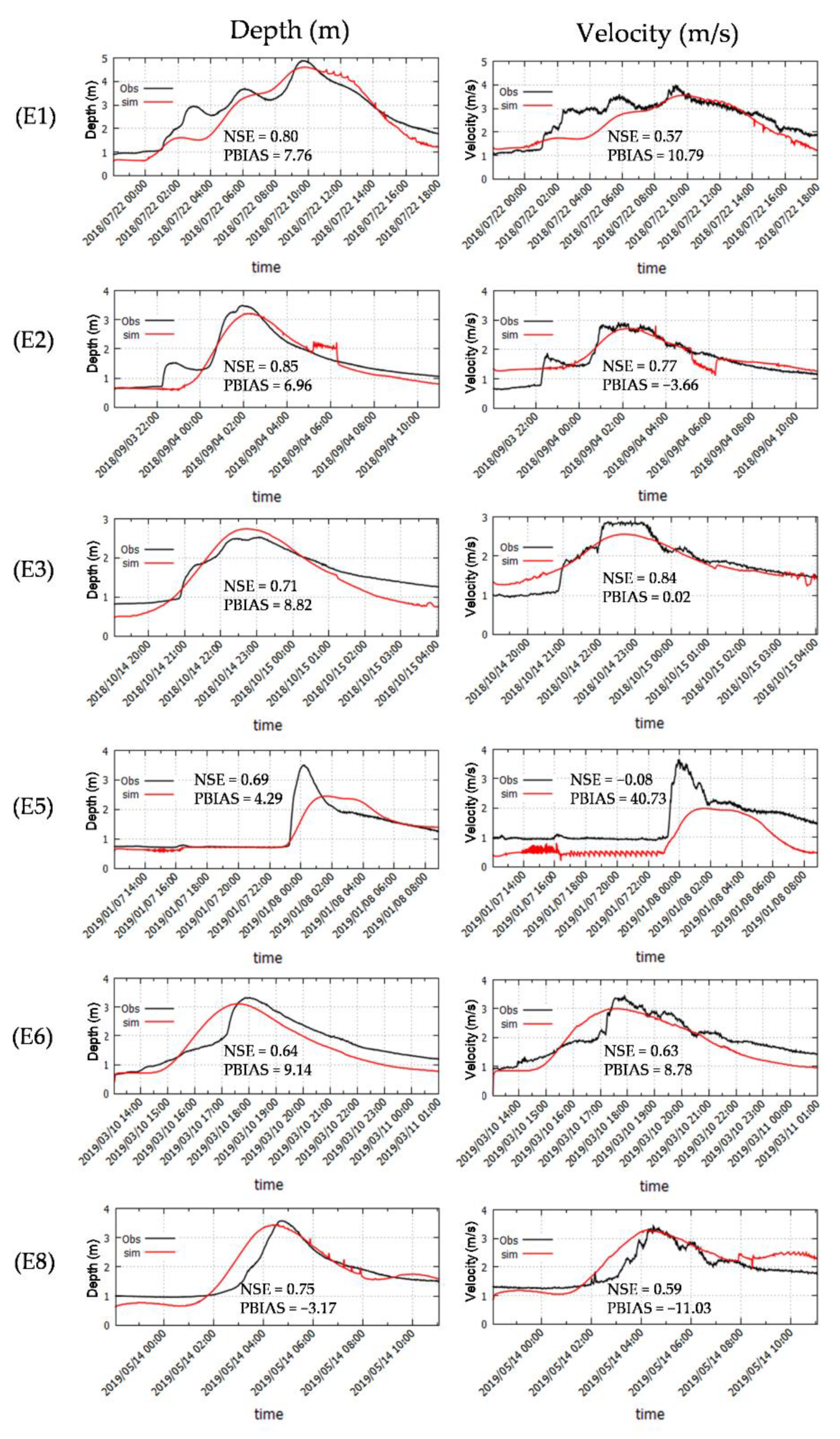
The Nays2DFlood showed satisfactory results in simulating water depths and flow velocity in the main channel (Figure 5). For the water depths over the calibration and validation events (E1-E3, E5, E6, E8), the NSE values ranged between 0.64 and 0.85, while the PBIAS varied from −3.17% to 8.62% (Figure 5). Overall, the model was able to simulate the magnitude and timing of the water depths with a general tendency to underestimate its magnitude by 5.6%, which represents ‘very good’ performance in conformity with the Moriasi et al. [21] performance ratings. For the flow velocity, the NSE (0.57–0.84) and the PBIAS (−11.03–10.79%) described a reasonable goodness-of-fit in five of the six evaluated events (E1-E3, E6, E8; Figure 5). The model was not able to recreate the water velocity during event E5 (NSE = −0.08; PBIAS = 40.73%; Figure 5). This error in the flow velocity was associated with the low accuracy of the hydrologic model in simulating the streamflow for this event due to the complexity of describing precipitation patterns across the study area with a single weather station. However, we believe these limitations can be overcome in the near future by improving the precipitation monitoring network in the study area and/or using remote sensing data.
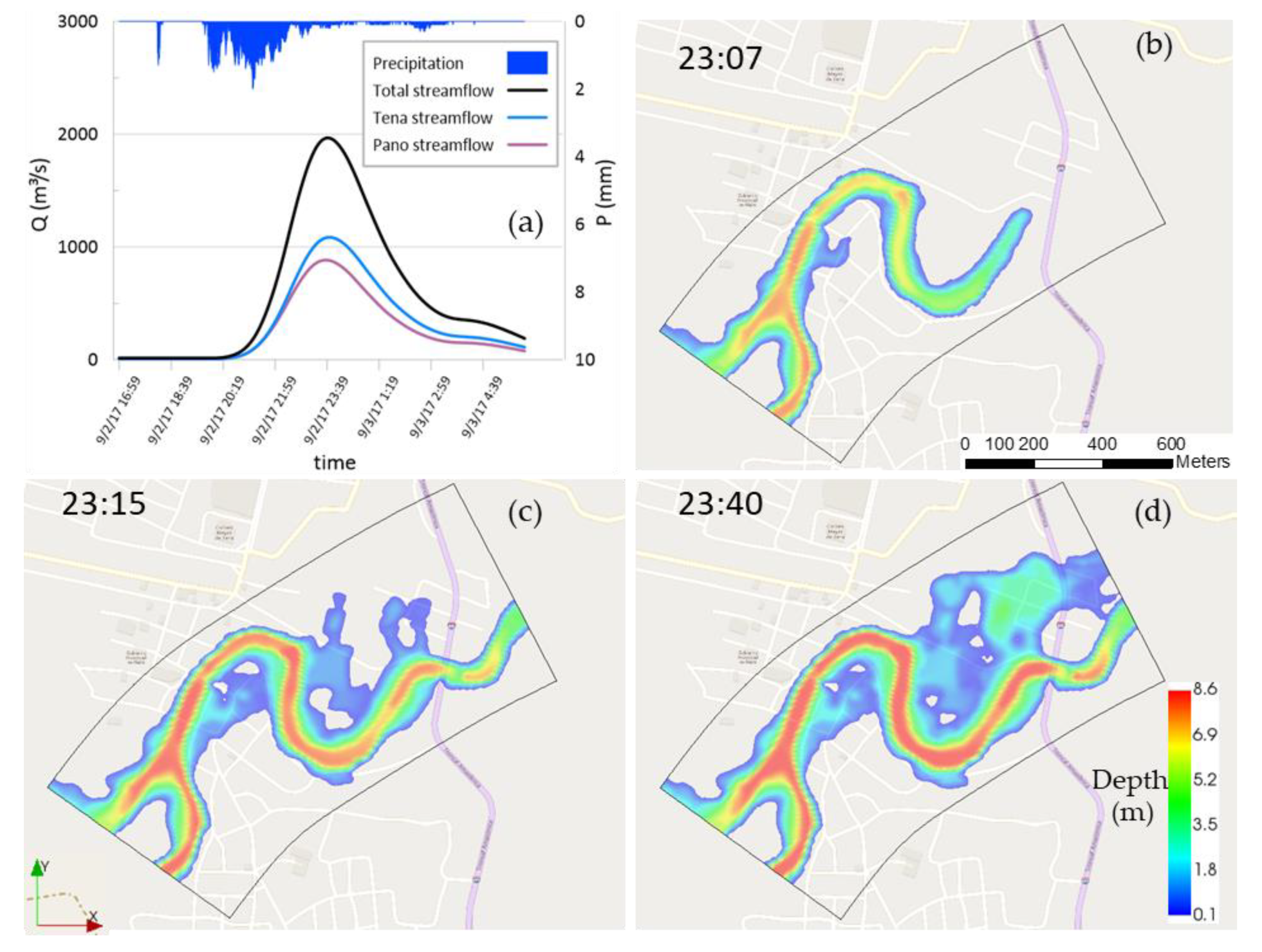
Given that there were no streamflow records for the precipitation event that flooded the city of Tena in September 2017, they were recreated using the calibrated HEC-HMS model (Figure 6a). At the junction of the Pano and Tena rivers, the simulated peak flow was equal to 1967 m3/s (Figure 6a), i.e., 5.1% less than that estimated by Fernandez and Bateman [57] for the same area based on the precipitation event that INAMHI described with a 500-year return period [51].
According to the simulation results, the river started overflowing 150 m downstream of the confluence of the Pano and Tena rivers at 23:07 (111 minutes after the peak precipitation was observed; Figure 6a,b), and only 8 minutes later (23:15), several river segments near the meanders were overflowing simultaneously. Moreover, when the peak flow was observed (23:40), most of the floodplains were almost covered. These results may help stakeholders to develop flood emergency plans that consider evacuation plans, the establishment of early warnings, the construction of levees, or urban planning strategies to relocate vulnerable communities.
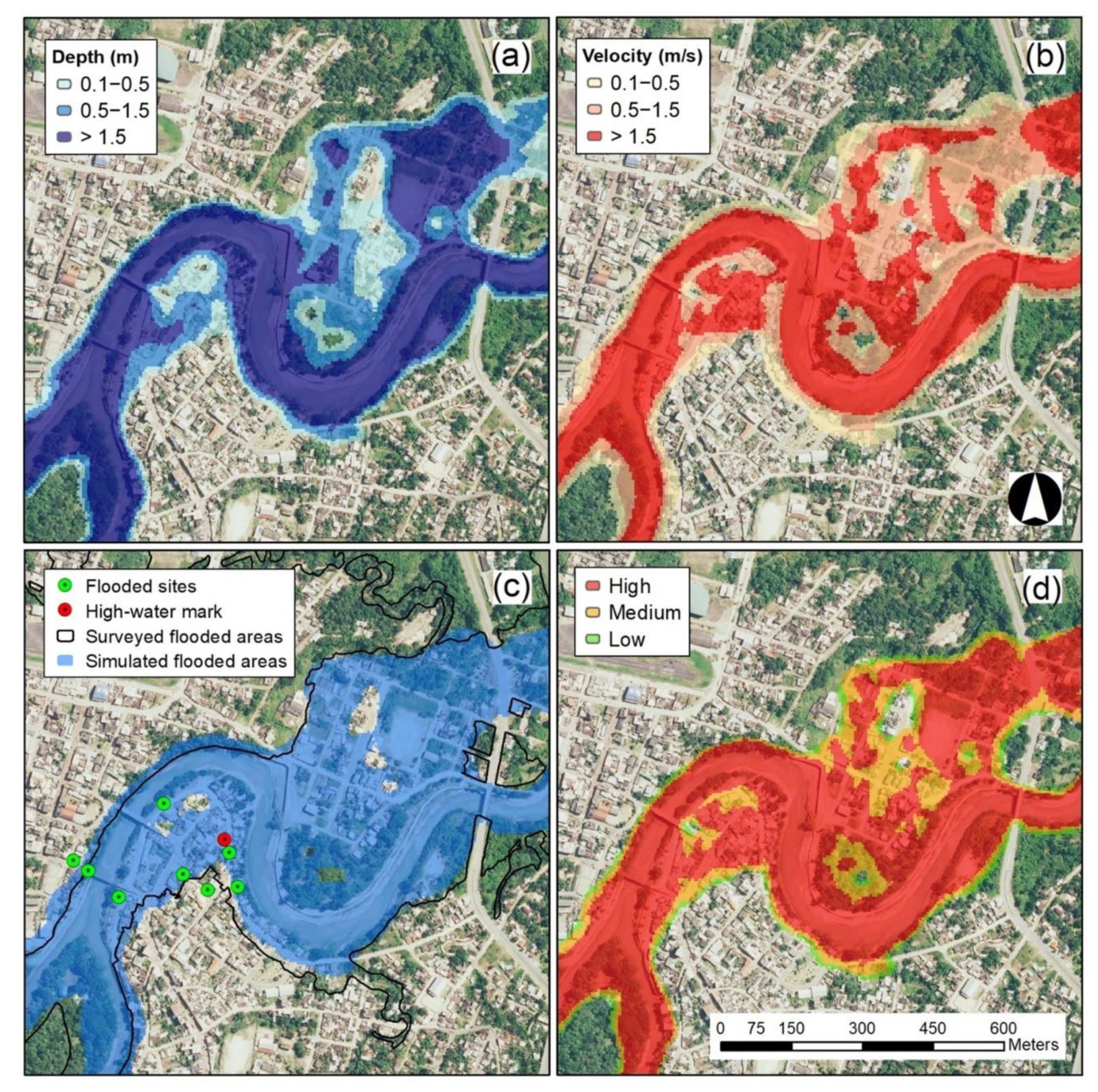
As mentioned in 2.4, the Nays2DFlood results were further validated using survey data of the flooded areas and control points of flooded sites. A high agreement between the simulated and observed flooded areas was obtained based on the fit index (F = 0.8). Additionally, six of the eight control points of flooded sites were within the simulated flooded areas, and the simulated water depth (1.23 m) matched that observed in a high-water mark (1.2 m) left on a building after the flood event (Figure 7c).
The values reported in Figure 7 correspond to the instant at which the peak flow in the channel was reached (11:40 pm; Figure 6a). The flood intensity map (Figure 7d) indicated that 71% of the flooded areas (40.9 ha) were under a high intensity, while 23% and 6% were under medium and low intensity, respectively. The flood intensity map also showed that the Bellavista and El Tereré neighborhoods were the most affected, being within high flood intensity areas (water depth > 1.5 m or flow velocity > 1.5 m/s). Accordingly, the maximum water depths in the floodplains were approximately 2 m and 4 m in the Bellavista and El Tereré neighborhoods, respectively, while the maximum water depth in the main channel was 8.5 m. The maximum flow velocity in the floodplains, on the other hand, was approximately 3 m/s across both neighborhoods, while in the main channel, a maximum of 9.4 m/s was reached (Figure 7). These areas with medium and high flood intensities may represent a threat to individuals and hinder evacuation and rescue tasks, given that at a water depth of at least 0.3 m and a flow velocity of 2.0 m/s, humans and cars become unstable [88,89]. Moreover, a water depth of 1.5 m may represent a damage factor of 0.84 on South American residential buildings [90]. Governmental reports stated that one person died and 1312 people, 324 houses, 36 private goods, and three public goods were affected during this extreme flood event [91].
4. Conclusions
This study coupled HEC-HMS and Nays2Dflood with event sampling and survey data to simulate the hydrologic response of data-scarce watersheds for a flood hazard assessment in the city of Tena. The results showed that this approach is suitable for calibrating and validating hydrologic and hydrodynamic models and recreating extreme flood events. Our modeling framework was reliable in simulating the streamflow and water depths of the main channel in 75% of the evaluated storm events, indicating that under certain conditions, data from a single precipitation gauge can accurately represent the spatio-temporal patterns of precipitation across the study area. Additionally, survey data such as polygons of flooded areas, control points of flooded sites, and high-water marks can provide sufficient information to constrain hydrodynamic models in the two-dimensional space. We appropriately reproduced an extreme flood event that occurred in September 2017 due to a 500-year precipitation event, where streamflow records were not available. According to our flood intensity map, 94% of the floodplains were under medium or high intensity, which may represent a threat to life, hinder evacuation and rescue tasks, and significantly damage residential and civil infrastructure.
The framework that we developed in this study facilitated the evaluation of the possible impacts of flood events on urban areas located in watersheds where robust monitoring networks are not available. Despite the assumptions that long-term data and multiple monitoring points are required for flood hazard assessment and the establishment of flood forecasting systems, we found that event sampling and survey data can cope with data scarcity and pave the way for flood research and the establishment of flood monitoring/forecasting systems in developing countries while their monitoring systems are being improved. This will enable stakeholders to formulate timely adaptation and mitigating plans to lessen the impacts of flood events at the local scale.
Author Contributions
Conceptualization, J.H.-P., F.J.-P., E.E.-S. and J.S.A.T.; Data curation, E.E.-S.; Formal analysis, J.H.-P.; Writing—original draft, J.H.-P. and F.J.-P.; Writing—review & editing, J.H.-P., F.J.-P., E.E.-S. and J.S.A.T. All authors have read and agreed to the published version of the manuscript.
Funding
This research received no external funding.
Acknowledgments
The authors would like to acknowledge Universidad Regional Amazónica Ikiam for providing access to its hydro-meteorological and survey data archive. Special thanks to Jorge Celi for his assistance for the development of this work. Also, authors would like to acknowledge the Municipality of Tena for providing information about flooded areas and the Secretary of Higher Education, Science, Technology, and Innovation for its financial support of the PhD scholarships of Jorge Hurtado and Fernando Jarrin. Lastly, the authors would like to acknowledge the reviewers of the manuscript for their valuable feedback.
Conflicts of Interest
The authors declare no conflict of interest.
References
- Jain, S.K.; Mani, P.; Jain, S.K.; Prakash, P.; Singh, V.P.; Tullos, D.; Kumar, S.; Agarwal, S.P.; Dimri, A.P. A Brief Review of Flood Forecasting Techniques and Their Applications. Int. J. River Basin Manag. 2018, 16, 329–344. [Google Scholar] [CrossRef]
- IPCC. AR5 Climate Change 2013: The Physical Science Basis—IPCC; Cambridge University Press: Cambridge, UK; New York, NY, USA, 2013; p. 1535. [Google Scholar]
- Merz, B.; Aerts, J.; Arnbjerg-Nielsen, K.; Baldi, M.; Becker, A.; Bichet, A.; Blöschl, G.; Bouwer, L.M.; Brauer, A.; Cioffi, F.; et al. Floods and Climate: Emerging Perspectives for Flood Risk Assessment and Management. Nat. Hazards Earth Syst. Sci. 2014, 14, 1921–1942. [Google Scholar] [CrossRef] [Green Version]
- Yin, J.; Gentine, P.; Zhou, S.; Sullivan, S.C.; Wang, R.; Zhang, Y.; Guo, S. Large Increase in Global Storm Runoff Extremes Driven by Climate and Anthropogenic Changes. Nat. Commun. 2018, 9, 4389. [Google Scholar] [CrossRef] [PubMed] [Green Version]
- Merkuryeva, G.; Merkuryev, Y.; Sokolov, B.V.; Potryasaev, S.; Zelentsov, V.A.; Lektauers, A. Advanced River Flood Monitoring, Modelling and Forecasting. J. Comput. Sci. 2015, 10, 77–85. [Google Scholar] [CrossRef]
- Díez-Herrero, A.; Huerta, L.L.; Isidro, M.L. A Handbook on Flood Hazard Mapping Methodologies; Geological Survey of Spain: Madrid, Spain, 2009. [Google Scholar]
- Bates, P.D.; De Roo, A.P.J. A Simple Raster-Based Model for Flood Inundation Simulation. J. Hydrol. 2000, 236, 54–77. [Google Scholar] [CrossRef]
- Shimizu, Y.; Inoue, T.; Suzuki, E.; Kawamura, S.; Iwasaki, T.; Hamaki, M.; Omura, K.; Kakegawa, E.; Yoshida, T. Nays2DFlood—Solver Manual; The International River Interface Cooperative (iRIC): Hokkaido, Japan, 2015; pp. 1–51. [Google Scholar]
- Bladé, E.; Cea, L.; Corestein, G.; Escolano, E.; Puertas, J.; Vázquez-Cendón, E.; Dolz, J.; Coll, A. Iber: Herramienta de Simulación Numérica Del Flujo En Ríos. Int. J. Numer. Methods Calc. Des. Eng. (RIMNI) 2014, 30, 1–10. [Google Scholar] [CrossRef] [Green Version]
- Fernández-Pato, J.; Caviedes-Voullième, D.; García-Navarro, P. Rainfall/Runoff Simulation with 2D Full Shallow Water Equations: Sensitivity Analysis and Calibration of Infiltration Parameters. J. Hydrol. 2016, 536, 496–513. [Google Scholar] [CrossRef]
- Smart, G.M. Improving Flood Hazard Prediction Models. Int. J. River Basin Manag. 2018, 16, 449–456. [Google Scholar] [CrossRef]
- Rai, P.K.; Dhanya, C.T.; Chahar, B.R. Coupling of 1D Models (SWAT and SWMM) with 2D Model (IRIC) for Mapping Inundation in Brahmani and Baitarani River Delta. Nat. Hazards 2018, 92, 1821–1840. [Google Scholar] [CrossRef]
- Hanif, A.; Dhanasekar, A.; Keene, A.; Li, H.; Carlson, K. Flood Risk Assessment Methodology for Planning under Climate Change Scenarios and the Corresponding Change in Land Cover. J. Water Clim. Chang. 2019. [Google Scholar] [CrossRef]
- Mishra, B.K.; Rafiei Emam, A.; Masago, Y.; Kumar, P.; Regmi, R.K.; Fukushi, K. Assessment of Future Flood Inundations under Climate and Land Use Change Scenarios in the Ciliwung River Basin, Jakarta. J. Flood Risk Manag. 2018, 11, S1105–S1115. [Google Scholar] [CrossRef]
- Liu, Z.; Zhang, H.; Liang, Q. A Coupled Hydrological and Hydrodynamic Model for Flood Simulation. Hydrol. Res. 2019, 50, 589–606. [Google Scholar] [CrossRef]
- Zhang, Y.; Zhou, J.; Lu, C. Integrated Hydrologic and Hydrodynamic Models to Improve Flood Simulation Capability in the Data-Scarce Three Gorges Reservoir Region. Water 2020, 12, 1462. [Google Scholar] [CrossRef]
- Chang, H.; Franczyk, J. Climate Change, Land-Use Change, and Floods: Toward an Integrated Assessment. Geogr. Compass 2008, 2, 1549–1579. [Google Scholar] [CrossRef]
- Barbedo, J.; Miguez, M.; van der Horst, D.; Marins, M. Enhancing Ecosystem Services for Flood Mitigation: A Conservation Strategy for Peri-Urban Landscapes? Ecol. Soc. 2014, 19, 54. [Google Scholar] [CrossRef]
- Tsakiris, G. Flood Risk Assessment: Concepts, Modelling, Applications. Nat. Hazards Earth Syst. Sci. 2014, 14, 1361–1369. [Google Scholar] [CrossRef] [Green Version]
- De Roo, A.; Schmuck, G.; Perdigao, V.; Thielen, J. The Influence of Historic Land Use Changes and Future Planned Land Use Scenarios on Floods in the Oder Catchment. Phys. Chem. Earth, Parts A/B/C 2003, 28, 1291–1300. [Google Scholar] [CrossRef]
- Moriasi, D.N.; Arnold, J.G.; Van Liew, M.W.; Bingner, R.L.; Harmel, R.D.; Veith, T.L.; Harmel, D.; Veith, T.L. Model Evaluation Guidelines for Systematic Quantification of Accuracy in Watershed Simulations. Trans. ASABE 2007, 50, 885–900. [Google Scholar] [CrossRef]
- Gupta, H.V.; Sorooshian, S.; Yapo, P.O. Status of Automatic Calibration for Hydrologic Models: Comparison with Multilevel Expert Calibration. J. Hydrol. Eng. 1999, 4, 135–143. [Google Scholar] [CrossRef]
- Teng, J.; Jakeman, A.J.J.; Vaze, J.; Croke, B.F.W.F.W.; Dutta, D.; Kim, S. Flood Inundation Modelling: A Review of Methods, Recent Advances and Uncertainty Analysis. Environ. Model. Softw. 2017, 90, 201–216. [Google Scholar] [CrossRef]
- Peña, F.; Nardi, F. Floodplain Terrain Analysis for Coarse Resolution 2D Flood Modeling. Hydrol. 2018, 5, 52. [Google Scholar] [CrossRef] [Green Version]
- Papaioannou, G.; Loukas, A.; Vasiliades, L.; Aronica, G.T. Flood Inundation Mapping Sensitivity to Riverine Spatial Resolution and Modelling Approach. Nat. Hazards 2016, 83, 117–132. [Google Scholar] [CrossRef]
- Caviedes-Voullième, D.; García-Navarro, P.; Murillo, J. Influence of Mesh Structure on 2D Full Shallow Water Equations and SCS Curve Number Simulation of Rainfall/Runoff Events. J. Hydrol. 2012, 448–449, 39–59. [Google Scholar] [CrossRef]
- Boongaling, C.G.K.; Faustino-Eslava, D.V.; Lansigan, F.P. Modeling Land Use Change Impacts on Hydrology and the Use of Landscape Metrics as Tools for Watershed Management: The Case of an Ungauged Catchment in the Philippines. Land Use Policy 2018, 72, 116–128. [Google Scholar] [CrossRef]
- Acero Triana, J.S.; Chu, M.L.; Guzman, J.A.; Moriasi, D.N.; Steiner, J.L. Beyond Model Metrics: The Perils of Calibrating Hydrologic Models. J. Hydrol. 2019, 578, 124032. [Google Scholar] [CrossRef]
- Johnston, R.; Smakhtin, V. Hydrological Modeling of Large River Basins: How Much Is Enough? Water Resour. Manag. 2014, 28, 2695–2730. [Google Scholar] [CrossRef] [Green Version]
- Reynolds, J.E.; Halldin, S.; Seibert, J.; Xu, C.Y.; Grabs, T. Robustness of Flood-Model Calibration Using Single and Multiple Events. Hydrol. Sci. J. 2019, 6667, 842–853. [Google Scholar] [CrossRef] [Green Version]
- McIntyre, N.; Lee, H.; Wheater, H.; Young, A.; Wagener, T. Ensemble Predictions of Runoff in Ungauged Catchments. Water Resour. Res. 2005, 41, 1–14. [Google Scholar] [CrossRef] [Green Version]
- Perrin, C.; Oudin, L.; Andreassian, V.; Rojas-Serna, C.; Michel, C.; Mathevet, T. Impact of Limited Streamflow Data on the Efficiency and the Parameters of Rainfall-Runoff Models. Hydrol. Sci. J. 2007, 52, 131–151. [Google Scholar] [CrossRef] [Green Version]
- Seibert, J.; McDonnell, J.J. Gauging the Ungauged Basin: Relative Value of Soft and Hard Data. J. Hydrol. Eng. 2015, 20, A4014004. [Google Scholar] [CrossRef] [Green Version]
- Correa, A.; Windhorst, D.; Crespo, P.; Célleri, R.; Feyen, J.; Breuer, L. Continuous versus Event-Based Sampling: How Many Samples Are Required for Deriving General Hydrological Understanding on Ecuador’s Páramo Region? Hydrol. Process. 2016, 30, 4059–4073. [Google Scholar] [CrossRef]
- Seibert, J.; Beven, K.J. Gauging the Ungauged Basin: How Many Discharge Measurements Are Needed? Hydrol. Earth Syst. Sci. 2009, 13, 883–892. [Google Scholar] [CrossRef] [Green Version]
- Juston, J.; Seibert, J.; Johansson, P.-O. Temporal Sampling Strategies and Uncertainty in Calibrating a Conceptual Hydrological Model for a Small Boreal Catchment. Hydrol. Process. 2009, 23, 3093–3109. [Google Scholar] [CrossRef]
- Espinoza, J.C.; Chavez, S.; Ronchail, J.; Junquas, C.; Takahashi, K.; Lavado, W. Rainfall Hotspots over the Southern Tropical Andes: Spatial Distribution, Rainfall Intensity, and Relations with Large-Scale Atmospheric Circulation. Water Resour. Res. 2015, 51, 3459–3475. [Google Scholar] [CrossRef]
- GAD-TENA. Actualización Plan de Desarrollo y Ordenamiento Territorial de Tena; Gobierno Municipal de Tena: Tena, Ecuador, 2014. [Google Scholar]
- Cruz-Cueva, G. Elaboración de Un Plan de Contingencia Por Inundación Del Río Tena En Los Barrios: Bellavista Las Hierbitas Tereré y Barrio Central de La Ciudad de Tena. PUCE: Quito, Ecuador, 2016. (In Spanish) [Google Scholar]
- Moreno, J.; Yerovi, F.; Herrera, M.; Yánez, D.; Espinosa, J.; Sánchez, D.; Merlo, J.; Haro, R.; Acosta, M.; Bernal, G. Soils from the Amazonia; Springer: Madison, WI, USA, 2018; pp. 79–111. [Google Scholar] [CrossRef]
- Tobón, C. Los Bosques Andinos y El Agua; ECOBONA: Quito, Ecuador, 2008. [Google Scholar]
- MAGAP-SIGTIERRAS. Generación de Geoinformación para la Gestión del Territorio a Nivel Nacional. Available online: metadatos.sigtierras.gob.ec (accessed on 12 July 2020). (In Spanish).
- Cadilhac, L.; Torres, R.; Calles, J.; Vanacker, V.; Calderón, E. Desafíos Para La Investigación Sobre El Cambio Climático En Ecuador. Neotrop. Biodivers. 2017, 3, 168–181. [Google Scholar] [CrossRef]
- INEC. Censo de Poblacion y Vivienda 2010. Available online: https://www.ecuadorencifras.gob.ec/estadisticas/ (accessed on 12 July 2020). (In Spanish).
- Palomino-Lemus, R.; Córdoba-Machado, S.; Gámiz-Fortis, S.R.; Castro-Díez, Y.; Esteban-Parra, M.J. Climate Change Projections of Boreal Summer Precipitation over Tropical America by Using Statistical Downscaling from CMIP5 Models. Environ. Res. Lett. 2017, 12, 124011. [Google Scholar] [CrossRef] [Green Version]
- Hirabayashi, Y.; Mahendran, R.; Koirala, S.; Konoshima, L.; Yamazaki, D.; Watanabe, S.; Kim, H.; Kanae, S. Global Flood Risk under Climate Change. Nat. Clim. Chang. 2013, 3, 816–821. [Google Scholar] [CrossRef]
- Sorribas, M.V.; Paiva, R.C.D.D.; Melack, J.M.; Bravo, J.M.; Jones, C.; Carvalho, L.; Beighley, E.; Forsberg, B.; Costa, M.H. Projections of Climate Change Effects on Discharge and Inundation in the Amazon Basin. Clim. Chang. 2016, 136, 555–570. [Google Scholar] [CrossRef]
- Armenta, E.; Villa, L.; Jácome, P. Proyecciones Climáticas De Precipitación Y Temperatura Para Ecuador, Bajo Distintos Escenarios De Cambio Climático.; Ministerio de Ambiente: Quito, Ecuador, 2016. (In Spanish) [Google Scholar]
- USGS. EarthExplorer. Available online: https://earthexplorer.usgs.gov/ (accessed on 6 June 2020).
- Sommer Messtechnick. RQ-30, RQ-30a, Discharge Measurement System User Manual.; Sommer GmbH: Koblach, Austria, 2014; Available online: https://www.sommer.at/en/products/water/rq-30-rq-30a (accessed on 12 July 2020).
- INAMHI. Determinación de Ecuaciones Para El Cálculo de Intensidades Máximas de Precipitación; Instituto Nacional de Meteorología e Hidrología (INAMHI): Quito, Ecuador, 2019; Available online: www.serviciometeorologico.gob.ec/Publicaciones/Hidrologia/ESTUDIO_DE_INTENSIDADES_V_FINAL.pdf (accessed on 12 July 2020). (In Spanish)
- Scharffenberg, B.; Bartles, M.; Braurer, T.; Fleming, M.; Karlovits, G. Hydrologic Modeling System HEC-HMS User’s Manual; No. 4.2; Hydrologic Engineering Center: Davis, CA, USA, 2016; Available online: https://www.hec.usace.army.mil/software/hec-hms/documentation/HEC-HMS_Users_Manual_4.2.pdf (accessed on 12 July 2020).
- Hawkins, R.H.; Ward, T.J.; Woodward, D.E.; Van Mullem, J.A. Curve Number Hydrology; American Society of Civil Engineers (ASCE): Reston, VA, USA, 2008. [Google Scholar]
- Cronshey, R. Urban Hydrology for Small Watersheds; U.S. Dept. of Agriculture Soil Conservation Service Engineering Division; United States Department of Agriculture (USDA): Washington, DC, USA, 1986. [Google Scholar]
- Merwade, V. Terrain Processing and HMS-Model Development Using GeoHMS Load the Data to ArcMap; Purdue University: West Lafayette, IN, USA, 2012; Available online: https://web.ics.purdue.edu/~vmerwade/education/geohms.pdf (accessed on 12 July 2020).
- Bondelid, T.R.; McCuen, R.H.; Jackson, T.J. Sensitivity of SCS Models to Curve Number Variation. J. Am. Water Resour. Assoc. 1982, 18, 111–116. [Google Scholar] [CrossRef]
- Fernandez Nualart, M.; Bateman Pinzon, A. Recuperación Paisajística y Estudio de Inundabilidad Del Sistema Hídrico a Su Paso Por Tena; Polytechnic University of Catalonia (UPC): Barcelona, Spain, 2004. (In Spanish) [Google Scholar]
- Vélez Upegui, J.J.; Botero Gutiérrez, A. Estimación Del Tiempo de Concentración y Tiempo de Rezago En La Cuenca Experimental Urbana de La Quebrada San Luis, Manizales. Dyna 2011, 165, 59. (In Spanish) [Google Scholar]
- Scharffenberg, W.A. Model Optimization. In Hydrologic Modeling System HEC-HMS, User Manual; US-Army-Corps-Engineers, Ed.; Hydrologic Engineering Center: Davis, CA, USA, 2016; pp. 383–419. [Google Scholar]
- Nash, J.E.; Sutcliffe, J.V. River Flow Forecasting through Conceptual Models Part I—A Discussion of Principles. J. Hydrol. 1970, 10, 282–290. [Google Scholar] [CrossRef]
- Shokory, J.A.N.; Tsutsumi, J.G.; Sakai, K. Flood Modeling and Simulation Using IRIC: A Case Study of Kabul City. E3S Web Conf. 2016, 7, 04003. [Google Scholar] [CrossRef] [Green Version]
- Kumar, S.; Kaushal, D.R.R.; Gosain, A.K.K. Hydrodynamic Simulation of Urban Stormwater Drain (Delhi City, India) Using IRIC Model. J. Appl. Res. Technol. 2018, 16, 67–78. [Google Scholar] [CrossRef] [Green Version]
- Chow, V. Hidráulica de Canales Abiertos; McGraw Hill: Bogotá, Colombia, 1994. (In Spanish) [Google Scholar]
- van der Sande, C.J.; de Jong, S.M.; de Roo, A.P.J. A Segmentation and Classification Approach of IKONOS-2 Imagery for Land Cover Mapping to Assist Flood Risk and Flood Damage Assessment. Int. J. Appl. Earth Obs. Geoinf. 2003, 4, 217–229. [Google Scholar] [CrossRef]
- Horritt, M.S.S.; Bates, P.D.D. Evaluation of 1D and 2D Numerical Models for Predicting River Flood Inundation. J. Hydrol. 2002, 268, 87–99. [Google Scholar] [CrossRef]
- Timbe, L.; Willems, P. Desempeño de Modelos Hidráulicos 1D y 2D Para La Simulación de Inundaciones. Maskana 2011, 2, 91–98. (In Spanish) [Google Scholar] [CrossRef]
- Domeneghetti, A.; Castellarin, A.; Tarpanelli, A.; Moramarco, T. Investigating the Uncertainty of Satellite Altimetry Products for Hydrodynamic Modelling. Hydrol. Process. 2015, 29, 4908–4918. [Google Scholar] [CrossRef]
- Ciervo, F.; Papa, M.N.; Medina, V.; Bateman, A. Simulation of Flash Floods in Ungauged Basins Using Post-Event Surveys and Numerical Modelling. J. Flood Risk Manag. 2015, 8, 343–355. [Google Scholar] [CrossRef]
- Mtamba, J.; van der Velde, R.; Ndomba, P.; Zoltán, V.; Mtalo, F. Use of Radarsat-2 and Landsat TM Images for Spatial Parameterization of Manning’s Roughness Coefficient in Hydraulic Modeling. Remote Sens. 2015, 7, 836–864. [Google Scholar] [CrossRef] [Green Version]
- Ponce, V.M. Kinematic Wave Controversy. J. Hydraul. Eng. 1991, 117, 511–525. [Google Scholar] [CrossRef]
- Barati, R.; Rahimi, S.; Akbari, G.H. Analysis of Dynamic Wave Model for Flood Routing in Natural Rivers. Water Sci. Eng. 2012, 5, 243–258. [Google Scholar] [CrossRef]
- Liu, Z.; Merwade, V.; Jafarzadegan, K. Investigating the Role of Model Structure and Surface Roughness in Generating Flood Inundation Extents Using One- and Two-Dimensional Hydraulic Models. J. Flood Risk Manag. 2019, 12, e12347. [Google Scholar] [CrossRef] [Green Version]
- Neto, A.; Batista, L.; Coutinho, R. Methodologies for Generation of Hazard Indicator Maps and Flood Prone Areas: Municipality of Ipojuca/PE. Rev. Bras. Recur. Hídricos 2016, 21, 377–390. [Google Scholar] [CrossRef]
- Courtel, F.; López, J.; Bello, M.; Noya, M. Mapas de Amenaza Por Inundaciones y Aludes Torrenciales En El Valle de Caracas. In Proceedings of the 32nd Congreso Latinoamericano De Hidráulica, Ciudad Guayana, Venezuela, 1−5 October 2006. (In Spanish). [Google Scholar]
- Cançado, V.; Brasil, L.; Nascimento, N.; Guerra, A. Flood Risk Assessment in an Urban Area: Measuring Hazard and Vulnerability. In Proceedings of the 11th International Conference on Urban Drainage, Edinburgh, Scotland, UK, 31 August–5 September 2008; IWA Publishing: Edinburgh, Scotland, UK, 2008; pp. 1–10. [Google Scholar]
- Da Silva, M.G.; De-Oliveira, A.; de Jesus Neves, R.J.; Nascimento, A.; Almeida, C.; Faccioli, G.G. Sensitivity Analysis and Calibration of Hydrological Modeling of the Watershed Northeast Brazil. J. Environ. Prot. 2015, 6, 837–850. [Google Scholar] [CrossRef] [Green Version]
- van Liew, M.W.; Arnold, J.G.; Bosch, D.D. Problems and Potential of Autocalibrating a Hydrologic Model. Trans. ASAE 2005, 48, 1025–1040. [Google Scholar] [CrossRef] [Green Version]
- Bin, L.; Xu, K.; Xu, X.; Lian, J.; Ma, C. Development of a Landscape Indicator to Evaluate the Effect of Landscape Pattern on Surface Runoff in the Haihe River Basin. J. Hydrol. 2018, 566, 546–557. [Google Scholar] [CrossRef]
- Asano, Y.; Uchida, T. The Roles of Channels and Hillslopes in Rainfall/Run-off Lag Times during Intense Storms in a Steep Catchment. Hydrol. Process. 2018, 32, 713–728. [Google Scholar] [CrossRef]
- Beven, K.; Binley, A. The Future of Distributed Models: Model Calibration and Uncertainty Prediction. Hydrol. Process. 1992, 6, 279–298. [Google Scholar] [CrossRef]
- Johnson, F.; White, C.J.; van Dijk, A.; Ekstrom, M.; Evans, J.P.; Jakob, D.; Kiem, A.S.; Leonard, M.; Rouillard, A.; Westra, S. Natural Hazards in Australia: Floods. Clim. Chang. 2016, 139, 21–35. [Google Scholar] [CrossRef] [Green Version]
- Iacob, O.; Brown, I.; Rowan, J. Natural Flood Management, Land Use and Climate Change Trade-Offs: The Case of Tarland Catchment, Scotland. Hydrol. Sci. J. 2017, 62, 1931–1948. [Google Scholar] [CrossRef] [Green Version]
- Bathurst, J.C.; Iroumé, A.; Cisneros, F.; Fallas, J.; Iturraspe, R.; Novillo, M.G.; Urciuolo, A.; de Bièvre, B.; Borges, V.G.; Coello, C.; et al. Forest Impact on Floods Due to Extreme Rainfall and Snowmelt in Four Latin American Environments 1: Field Data Analysis. J. Hydrol. 2011, 400, 281–291. [Google Scholar] [CrossRef]
- Dadson, S.J.; Hall, J.W.; Murgatroyd, A.; Acreman, M.; Bates, P.; Beven, K.; Heathwaite, L.; Holden, J.; Holman, I.P.; Lane, S.N.; et al. A Restatement of the Natural Science Evidence Concerning Catchment-Based ‘Natural’ Flood Management in the UK. Proc. R. Soc. A Math. Phys. Eng. Sci. 2017, 473, 20160706. [Google Scholar] [CrossRef] [Green Version]
- Hejl, H.; Kans, L. Roughness Coefficient for Flooded Urban Areas. J. Res. U.S. Geol. Surv. 1977, 5, 541–545. [Google Scholar]
- Mosquera-Machado, S.; Ahmad, S. Flood Hazard Assessment of Atrato River in Colombia. Water Resour. Manag. 2007, 21, 591–609. [Google Scholar] [CrossRef]
- Arcement, G.; Schneider, V. Guide for Selecting Manning’s Roughness Coefficients for Natural Channels and Flood Plains; United States Geological Survey (USGS): Denver, CO, USA, 1989.
- Xia, J.; Falconer, R.A.; Lin, B.; Tan, G. Numerical Assessment of Flood Hazard Risk to People and Vehicles in Flash Floods. Environ. Model. Softw. 2011, 26, 987–998. [Google Scholar] [CrossRef]
- Bocanegra, R.A.; Vallés-Morán, F.J.; Francés, F. Review and Analysis of Vehicle Stability Models during Floods and Proposal for Future Improvements. J. Flood Risk Manag. 2020, 13. [Google Scholar] [CrossRef] [Green Version]
- Huizinga, J.; de Moel, H.; Szewczyk, W. Glob. Flood Depth-Damage Functions: Methodology and the database with guidelines; Publications Office of the European Union: Luxemburg, 2017. [Google Scholar] [CrossRef]
- Servicio Nacional de Gestión de Riesgos y Emergencias (SNGRE). COE Cantonal Toma Resoluciones Ante emergencia en Tena. Boletín de Prensa. Available online: https://www.gestionderiesgos.gob.ec/coe-cantonal-toma-resoluciones-ante-emergencia-en-tena/ (accessed on 25 August 2020). (In Spanish).
Figure 1.
General features of the study area. (a) Location of the Napo province in Ecuador; (b) study area within the Napo province; (c) terrain elevation and location of the precipitation and streamflow gauges; (d) domain used for flood hazard assessment (red polygon) in the city of Tena.
Figure 1.
General features of the study area. (a) Location of the Napo province in Ecuador; (b) study area within the Napo province; (c) terrain elevation and location of the precipitation and streamflow gauges; (d) domain used for flood hazard assessment (red polygon) in the city of Tena.

Figure 2.
Time series of precipitation (P) and streamflow (Q) from July 2018 to May 2019. The orange dashed line represents the 211 m3/s threshold for storm event selection.
Figure 2.
Time series of precipitation (P) and streamflow (Q) from July 2018 to May 2019. The orange dashed line represents the 211 m3/s threshold for storm event selection.

Figure 3.
Hydrodynamic domain and control points for calibration and validation. (a) Modeling domain for the hydrodynamic simulations and location of the streamflow gauging station; (b) Polygon of flooded areas (black line), additional control points of flooded sites (greenish dots), and high-water mark (reddish dot) used to validate the results of the hydrodynamic model in simulating the 2017 flood event.

Figure 4.
Observed (black line) and simulated (red line) streamflow (m3/s) for the calibration and validation events (E1-E8).
Figure 4.
Observed (black line) and simulated (red line) streamflow (m3/s) for the calibration and validation events (E1-E8).

Figure 5.
Observed (black line) and simulated (reddish line) water depth (m) and flow velocity (m/s) for the calibration and validation events (E1-E3, E5, E6, E8).
Figure 5.
Observed (black line) and simulated (reddish line) water depth (m) and flow velocity (m/s) for the calibration and validation events (E1-E3, E5, E6, E8).

Figure 6.
Spatio-temporal evolution of the flood event generated by the 500-year storm on 2 September 2017. (a) HEC-HMS-reconstructed hydrograph. Flood stage (b) at the beginning of the river overflow, (c) when the overflow took place along several river segments, and (d) at the time of peak flow.
Figure 6.
Spatio-temporal evolution of the flood event generated by the 500-year storm on 2 September 2017. (a) HEC-HMS-reconstructed hydrograph. Flood stage (b) at the beginning of the river overflow, (c) when the overflow took place along several river segments, and (d) at the time of peak flow.

Figure 7.
Reconstructed 500-year flood event. (a) water depths; (b) flow velocities; (c) simulated flood extent against surveyed flooded areas (black line) and control points of flooded sites (greenish dots), and location of the high-water mark (reddish dot); (d) flood intensity map as a function of flow velocity and water depth in compliance with Cançado et al. [75] guidelines (Table 3).


Table 1.
Morphological and hydrological parameters of PRB and TRB.
| Parameter | Description [Units] | PRB | TRB |
|---|---|---|---|
| A | Drainage area [km2] | 99.96 | 134.86 |
| P | Perimeter [km] | 54.97 | 54.13 |
| El_min | Minimum elevation [m] | 499.00 | 499.00 |
| El_max | Maximum elevation [m] | 2494.00 | 2448.00 |
| El_ave | Mean elevation [m] | 982.00 | 1087.00 |
| Sl_min | Minimum slope [%] | 0.00 | 0.00 |
| Sl_max | Maximum slope [%] | 95.93 | 106.23 |
| Sl_ave | Mean slope [%] | 24.09 | 27.51 |
| Lh | Hydraulic length [km] | 25.43 | 27.99 |
| Le | Equivalent length [km] | 23.17 | 20.48 |
| Lr | Relative length of the largest reach (Lh / A^0.5) [-]; Lr > 1: elongated basin, Lr < 1: basins prone to floods | 2.54 | 2.41 |
| CN | Curve number for saturated conditions [-] | 90.00 | 87.00 |
| Tc | Time of concentration [minutes] | 180.00 | 190.00 |
| Lag | Lag time [minutes] | 108.00 | 114.00 |
| Bf | Baseflow [m3/s] | 6.00 | 9.00 |
Table 2.
Duration and peak flow of the eight storm events considered for model calibration and validation.
Table 2.
Duration and peak flow of the eight storm events considered for model calibration and validation.
| Event | Start (Date, Time) | End (Date, Time) | Duration (Hours) | Peak Flow (m3/s) |
|---|---|---|---|---|
| E1 | 21 July 2018, 12:00 | 23 July 2018, 12:00 | 48 | 714.20 |
| E2 | 03 September 2018, 12:00 | 04 September 2018, 18:00 | 30 | 356.00 |
| E3 | 14 October 2018, 12:00 | 15 October 2018, 08:00 | 20 | 234.80 |
| E4 | 24 November 2018, 00:00 | 24 November 2018, 24:00 | 24 | 403.30 |
| E5 | 07 January 2019, 12:00 | 08 January 2019, 12:00 | 24 | 435.60 |
| E6 | 10 March 2019, 06:00 | 11 March 2019, 06:00 | 24 | 395.60 |
| E7 | 27 April 2019, 00:00 | 27 April 2019, 24:00 | 24 | 589.80 |
| E8 | 13 May 2019, 00:00 | 14 May 2019, 24:00 | 48 | 424.40 |
Table 3.
Flood intensity as a function of flow velocities and water depth.
| Flood Intensity | Depth (D) [m]-Velocity (V) [m/s] |
|---|---|
| High | D > 1.5 or V > 1.5 |
| Medium | 0.5 < D < 1.5 or 0.5 < V < 1.5 |
| Low | 0.1 < D < 0.5 and 0.1 < V < 0.5 |
Table 4.
Observed and simulated peak flow, time at peak, and runoff volume for events E1-E8.
| Event | Observed | Simulated | ||||
|---|---|---|---|---|---|---|
| Time at Peak (Time) | Peak Flow (m3/s) | Runoff Volume (mm) | Time at Peak (Time) | Peak Flow (m3/s) | Runoff Volume (mm) | |
| E1 | 09:24 | 714.20 | 100.66 | 09:47 | 641.10 | 83.96 |
| E2 | 01:49 | 356.00 | 25.34 | 02:16 | 306.30 | 24.52 |
| E3 | 23:09 | 234.80 | 16.92 | 22:42 | 263.70 | 17.54 |
| E4 | 11:19 | 403.30 | 30.25 | 11:33 | 760.80 | 43.94 |
| E5 | 00:09 | 435.60 | 24.1 | 01:36 | 178.10 | 18.45 |
| E6 | 17:54 | 395.60 | 25.21 | 17:36 | 319.90 | 22.57 |
| E7 | 14:24 | 589.80 | 33.76 | 14:53 | 178.10 | 14.63 |
| E8 | 04:40 | 424.40 | 48.01 | 04:24 | 404.60 | 49.67 |
© 2020 by the authors. Licensee MDPI, Basel, Switzerland. This article is an open access article distributed under the terms and conditions of the Creative Commons Attribution (CC BY) license (http://creativecommons.org/licenses/by/4.0/).
Share and Cite
MDPI and ACS Style
Hurtado-Pidal, J.; Acero Triana, J.S.; Espitia-Sarmiento, E.; Jarrín-Pérez, F. Flood Hazard Assessment in Data-Scarce Watersheds Using Model Coupling, Event Sampling, and Survey Data. Water 2020, 12, 2768. https://doi.org/10.3390/w12102768
AMA Style
Hurtado-Pidal J, Acero Triana JS, Espitia-Sarmiento E, Jarrín-Pérez F. Flood Hazard Assessment in Data-Scarce Watersheds Using Model Coupling, Event Sampling, and Survey Data. Water. 2020; 12(10):2768. https://doi.org/10.3390/w12102768
Chicago/Turabian StyleHurtado-Pidal, Jorge, Juan S. Acero Triana, Edgar Espitia-Sarmiento, and Fernando Jarrín-Pérez. 2020. "Flood Hazard Assessment in Data-Scarce Watersheds Using Model Coupling, Event Sampling, and Survey Data" Water 12, no. 10: 2768. https://doi.org/10.3390/w12102768
Note that from the first issue of 2016, this journal uses article numbers instead of page numbers. See further details here.