Compound Inundation Impacts of Coastal Climate Change: Sea-Level Rise, Groundwater Rise, and Coastal Precipitation

 ,
,
Abstract
:1. Introduction
2. Methods
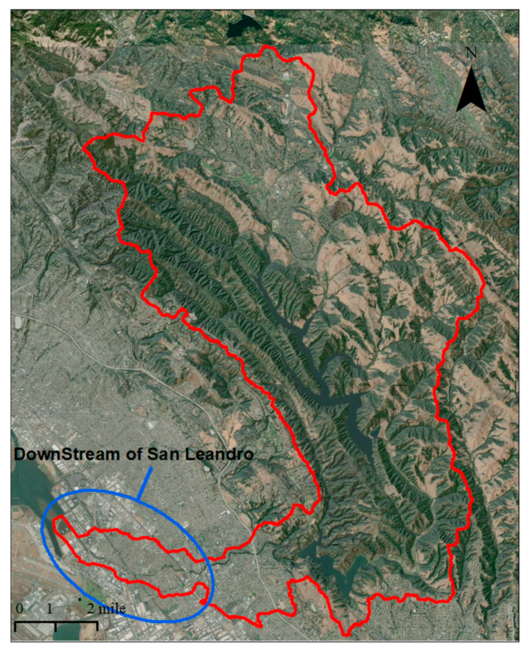
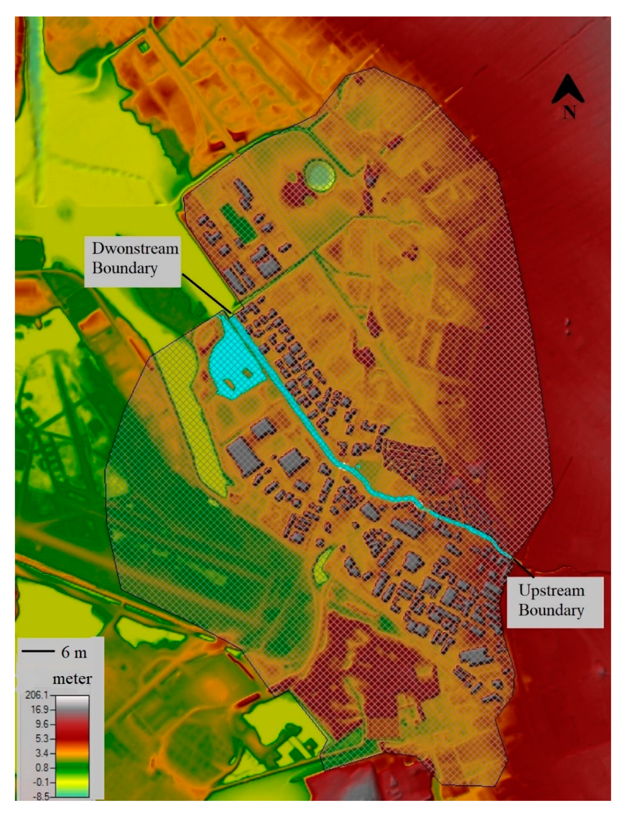
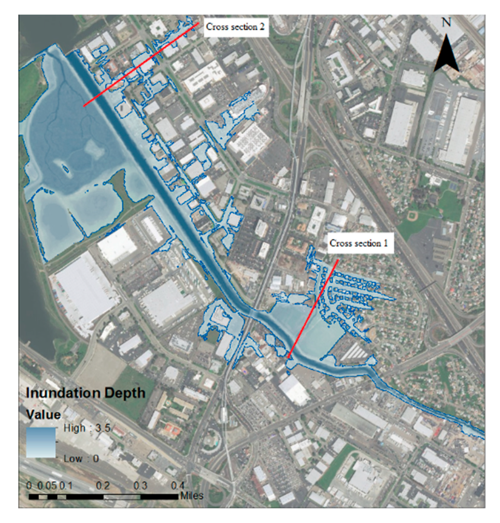
2.1. Study Area
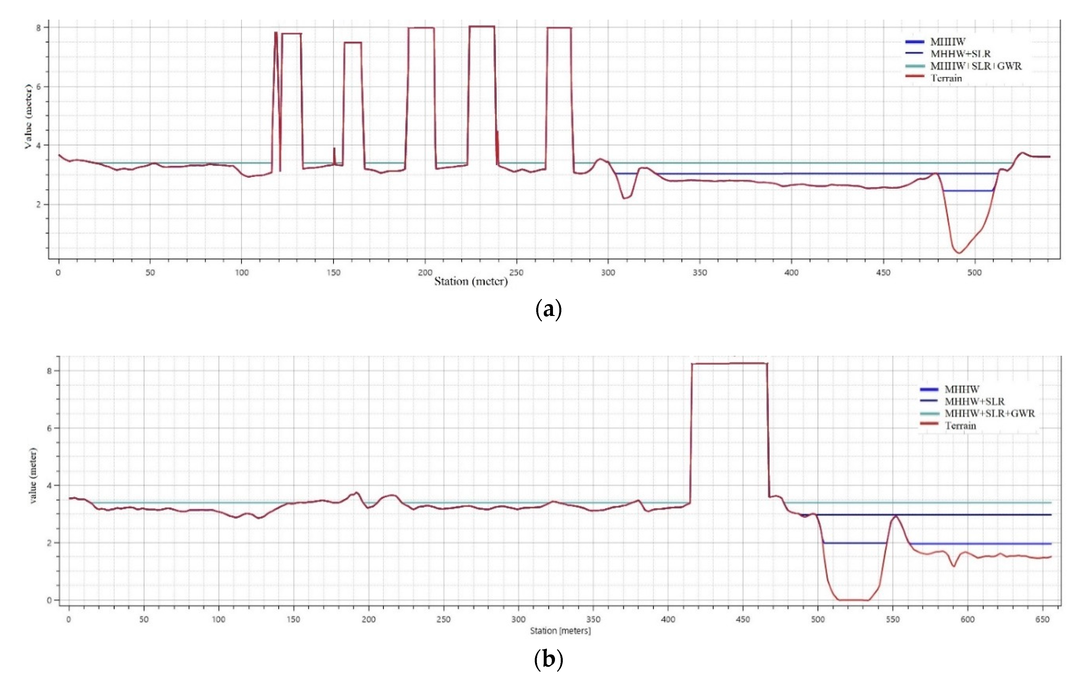
- In the first scenario, the value of MHHW (mean higher high water) which is 1.94 m is used as downstream boundary condition [48];
- In the second scenario 1 m SLR is added to MHHW value; and
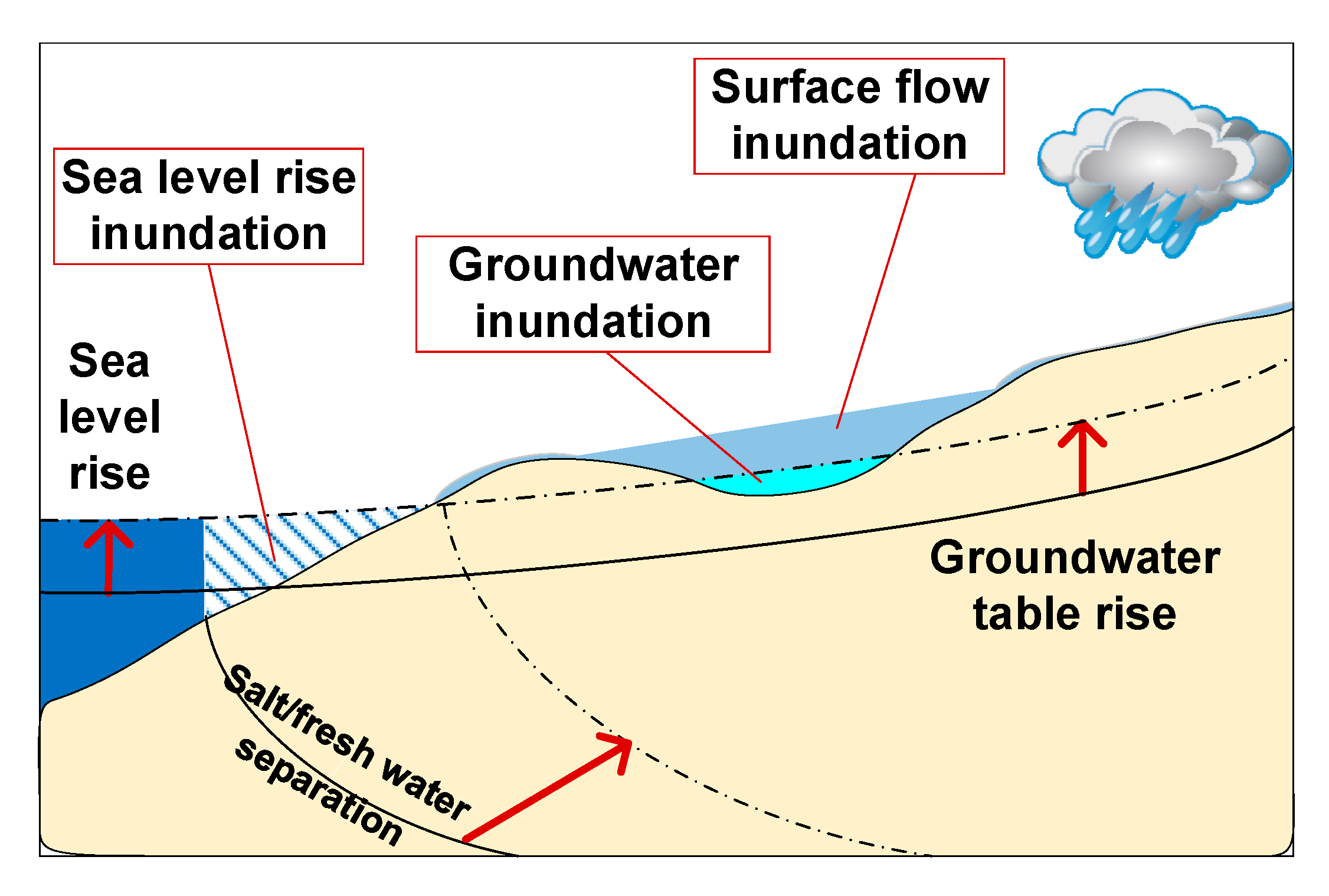
- In the third scenario groundwater inundation is also considered as a downstream boundary condition.
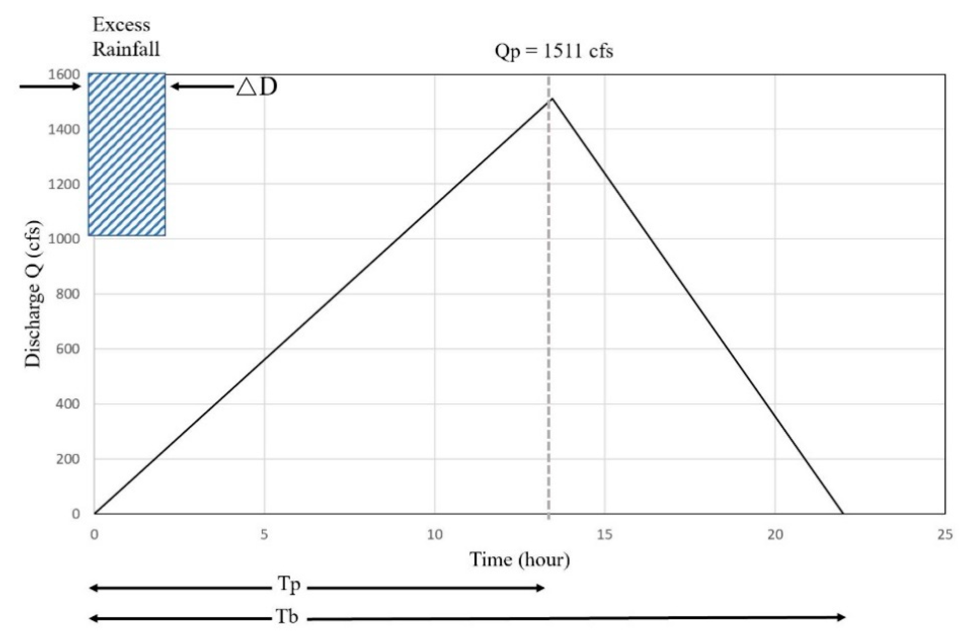
2.2. Modelling
3. Results
4. Discussion
5. Conclusions
Author Contributions
Funding
Conflicts of Interest
References
- Revell, D.L.; King, P.; Snyder, A.; Calil, J.; Gilliam, J.; Slaven, C.; Hart, J.; Boudreau, D.; Nakagawa, J.; Mercer, R.; et al. 2016 City of Imperial Beach Sea Level Rise Assessment; Coastal Conservancy: Imperial Beach, CA, USA, 2016.
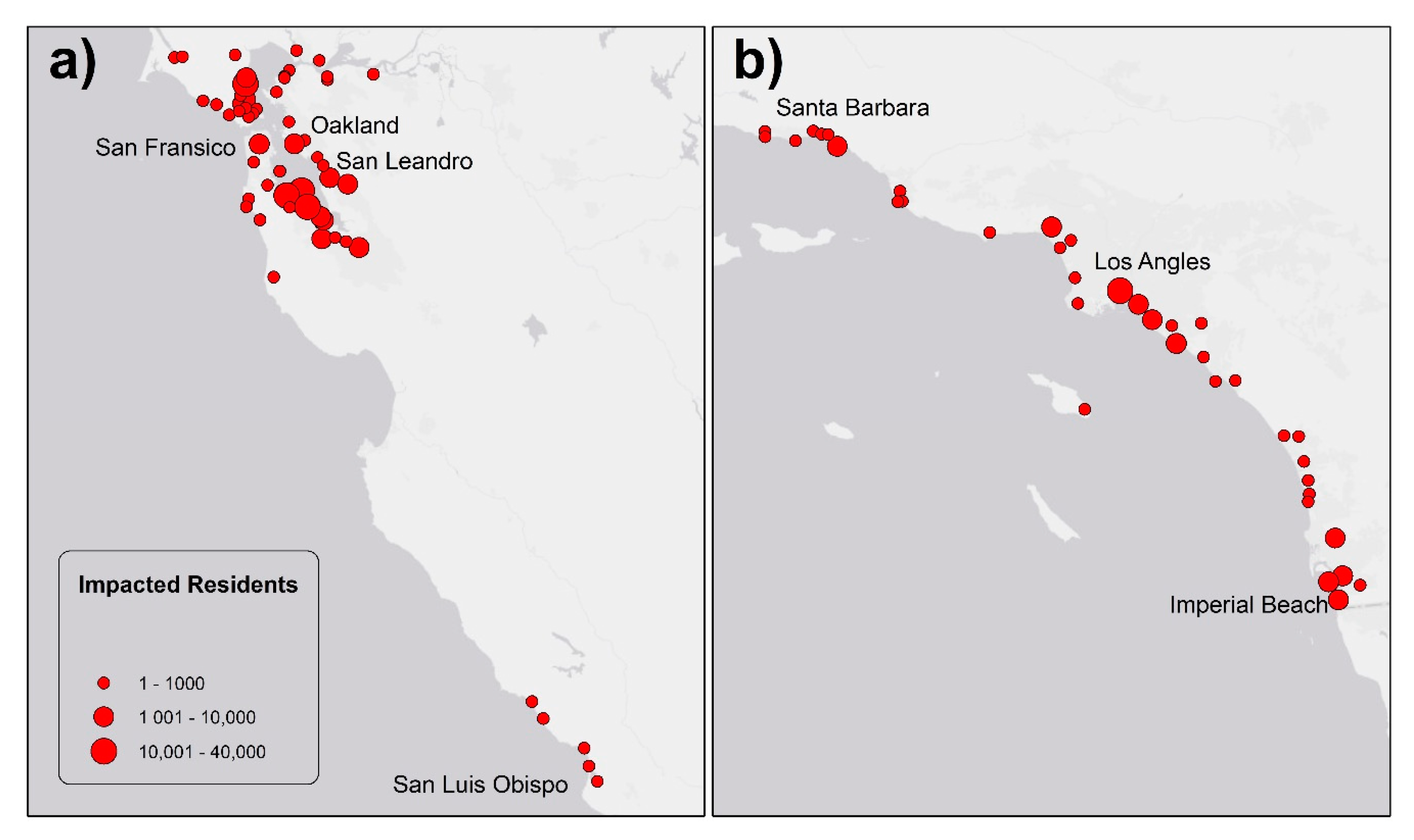
- Jones, J.M.; Wood, N.; Ng, P.; Henry, K.; Jones, J.L.; Peters, J.; Jamieson, M. Community Exposure in California to Coastal Flooding Hazards Enhanced by Climate Change; U.S. Geological Survey: Liston, VA, USA, 2016.
- Scavia, D.; Field, C.J.; Boesch, F.D.; Buddemeier, W.R.; Burkett, V.; Cayan, R.D.; Fogarty, M.; Harwell, A.M.; Howarth, W.R.; Mason, C.; et al. Climate change impacts on US coastal and marine ecosystems. Estuaries 2002, 25, 149–164. [Google Scholar] [CrossRef]
- Cayan, D.R.; Bromirski, P.D.; Hayhoe, K.; Tyree, M.; Dettinger, M.D.; Flick, R.E. Climate change projections of sea level extremes along the California coast. Clim. Chang. 2008, 87, 57–73. [Google Scholar] [CrossRef]
- Rahmstorf, S. A semi-empirical approach to projecting future sea-level rise. Science 2007, 315, 368–370. [Google Scholar] [CrossRef] [Green Version]
- Mastrandrea, M.D.; Luers, A.L. Climate change in California: Scenarios and approaches for adaptation. Clim. Chang. 2012, 111, 5–16. [Google Scholar] [CrossRef]
- Bindoff, L.N.; Willebrand, J.; Artale, V.; Cazenave, A.; Gregory, M.J.; Gulev, S.; Hanawa, K.; le Quere, C.; Levitus, S.; Nojiri, Y. Observations: Oceanic Climate Change and Sea Level; Cambridge University Press: Cambridge, UK, 2007. [Google Scholar]
- Hauer, M.E.; Evans, J.M.; Mishra, D.R. Millions projected to be at risk from sea-level rise in the continental United States. Nat. Clim. Chang. 2016, 6, 691–695. [Google Scholar] [CrossRef]
- Crossett, K.M.; Culliton, T.J.; Wiley, P.C.; Goodspeed, T.R. Population Trends along the Coastal United States: 1980–2008; US Department of Commerce: Columbia, WA, USA; National Oceanic: Silver Spring, MD, USA; Atmospheric Administration: Silver Spring, MD, USA, 2004; Volume 55.
- Heberger, M.; Cooley, H.; Herrera, P.; Gleick, P.H.; Moore, E. The Impacts of Sea-Level Rise on the California Coast; California Climate Change Center: San Diego, CA, USA, 2009.
- Bureau, U.S.C. State and county quickfacts. In Data derived from Population Estimates, American Community Survey, Census of Population and Housing, County Business Patterns, Economic Census, Survey of Business Owners, Building Permits; Consolidated Federal Funds Report; Census of Governments: Burbank, CA, USA, 2013. [Google Scholar]
- Arkema, K.K.; Guannel, G.; Verutes, G.; Wood, S.A.; Guerry, A.; Ruckelshaus, M.; Kareiva, P.; Lacayo, M.; Silver, J.M. Coastal habitats shield people and property from sea-level rise and storms. Nat. Clim. Chang. 2013, 3, 913–918. [Google Scholar] [CrossRef]
- Dawson, R.J.; Dickson, M.E.; Nicholls, R.J.; Hall, J.W.; Walkden, M.J.A.; Stansby, P.K.; Mokrech, M.; Richards, J.; Zhou, J.; Milligan, J.; et al. Integrated analysis of risks of coastal flooding and cliff erosion under scenarios of long term change. Clim. Chang. 2009, 95, 249–288. [Google Scholar] [CrossRef] [Green Version]
- Rotzoll, K.; Fletcher, C.H. Assessment of groundwater inundation as a consequence of sea-level rise. Nat. Clim. Chang. 2013, 3, 477–481. [Google Scholar] [CrossRef]
- Wahl, T.; Jain, S.; Bender, J.; Meyers, S.D.; Luther, M.E. Increasing risk of compound flooding from storm surge and rainfall for major US cities. Nat. Clim. Chang. 2015, 5, 1093–1097. [Google Scholar] [CrossRef]
- Hanson, R.T.; Izbicki, J.A.; Reichard, E.G.; Edwards, B.D.; Land, M.; Martin, P. Comparison of groundwater flow in Southern California coastal aquifers. Earth Sci. Urban Ocean. South. Calif. Cont. Borderl. 2009, 454, 345. [Google Scholar]
- Nishikawa, T.; Siade, A.J.; Reichard, E.G.; Ponti, D.J.; Canales, A.G.; Johnson, T.A. Stratigraphic controls on seawater intrusion and implications for groundwater management, Dominguez Gap area of Los Angeles, California, USA. Hydrogeol. J. 2009, 17, 1699. [Google Scholar] [CrossRef]
- Barlow, P.M.; Reichard, E.G. Saltwater intrusion in coastal regions of North America. Hydrogeol. J. 2010, 18, 247–260. [Google Scholar] [CrossRef]
- Kostigen, T.M. Could California’s drought last 200 years. Natl. Geogr. Retrieved 2014, 2, 2014. [Google Scholar]
- Lynn, E. California Climate Science and Data—for Water Resources Management; California Department of Water Resources: Sacramento, CA, USA, 2015.
- Zektser, S.; Loáiciga, H.A.; Wolf, J.T. Environmental impacts of groundwater overdraft: Selected case studies in the southwestern United States. Environ. Geol. 2005, 47, 396–404. [Google Scholar] [CrossRef]
- Werner, A.D.; Simmons, C.T. Impact of sea-level rise on sea water intrusion in coastal aquifers. Groundwater 2009, 47, 197–204. [Google Scholar] [CrossRef]
- Plane, E.; Hill, K.; May, C. A Rapid Assessment Method to Identify Potential Groundwater Flooding Hotspots as Sea Levels Rise in Coastal Cities. Water 2019, 11, 2228. [Google Scholar] [CrossRef] [Green Version]
- Bjerklie, D.M.; Mullaney, J.R.; Stone, J.R.; Skinner, B.J.; Ramlow, M.A. Preliminary Investigation of the Effects of Sea-Level Rise on Groundwater Levels in New Haven; US Geological Survey: Reston, VA, USA, 2012.
- Habel, S.; Fletcher, C.H.; Rotzoll, K.; El-Kadi, A.I. Development of a model to simulate groundwater inundation induced by sea-level rise and high tides in Honolulu. Hawaii Water Res. 2017, 114, 122–134. [Google Scholar] [CrossRef]
- Befus, K.M.; Barnard, P.L.; Hoover, D.J.; Finzi Hart, J.A.; Voss, C.I. Increasing threat of coastal groundwater hazards from sea-level rise in California. Nat. Clim. Chang. 2020. [Google Scholar] [CrossRef]
- Davtalab, R.; Mirchi, A.; Harris, R.J.; Troilo, M.X.; Madani, K. Sea Level Rise Effect on Groundwater Rise and Stormwater Retention Pond Reliability. Water 2020, 12, 1129. [Google Scholar] [CrossRef] [Green Version]
- Sadegh, M.; Moftakhari, H.; Gupta, H.V.; Ragno, E.; Mazdiyasni, O.; Sanders, B.; Matthew, R.; Aghakouchak, A. Multihazard scenarios for analysis of compound extreme events. Geophys. Res. Lett. 2018, 45, 5470–5480. [Google Scholar] [CrossRef] [Green Version]
- Sadegh, M.; Moftakhari, H.; Gupta, H.V.; Ragno, E.; Mazdiyasni, O.; Sanders, B.; Matthew, R.; Aghakouchak, A. Extreme precipitation events in the western United States related to tropical forcing. J. Clim. 2000, 13, 793–820. [Google Scholar]
- Karamouz, M.; Zahmatkesh, Z.; Goharian, E.; Nazif, S. Combined Impact of Inland and Coastal Floods: Mapping Knowledge Base for Development of Planning Strategies. J. Water Resour. Plan. Manag. 2015, 141, 04014098. [Google Scholar] [CrossRef]
- Moftakhari, H.R.; Salvadori, G.; Aghakouchak, A.; Sanders, B.F.; Matthew, R.A. Compounding effects of sea level rise and fluvial flooding. Proc. Natl. Acad. Sci. USA 2017, 114, 9785–9790. [Google Scholar] [CrossRef] [PubMed] [Green Version]
- Muñoz, D.F.; Moftakhari, H.; Moradkhani, H. Compound Effects of Flood Drivers and Wetland Elevation Correction on Coastal Flood Hazard Assessment. Water Resour. Res. 2020, 56, e2020WR027544. [Google Scholar] [CrossRef]
- Strauss, B.H.; Ziemlinski, R.; Weiss, J.L.; Overpeck, J.T. Tidally adjusted estimates of topographic vulnerability to sea level rise and flooding for the contiguous United States. Environ. Res. Lett. 2012, 7, 014033. [Google Scholar] [CrossRef]
- Sukop, M.C.; Rogers, M.; Guannel, G.; Infanti, J.M.; Hagemann, K. High temporal resolution modeling of the impact of rain, tides, and sea level rise on water table flooding in the Arch Creek basin, Miami-Dade County Florida USA. Sci. Total Environ. 2018, 616–617, 1668–1688. [Google Scholar] [CrossRef] [PubMed]
- Quirogaa, V.M.; Kurea, S.; Udoa, K.; Manoa, A. Application of 2D numerical simulation for the analysis of the February 2014 Bolivian Amazonia flood: Application of the new HEC-RAS version 5. Ribagua 2016, 3, 25–33. [Google Scholar] [CrossRef] [Green Version]
- Srinivas, K.; Werner, M.; Wright, N. Comparing Forecast Skill of Inundation Models of Differing Complexity: The Case of Upton upon Severn; Taylor & Francis Group: London, UK, 2009; pp. 85–94. [Google Scholar]
- Poretti, I.; de Amicis, M. An approach for flood hazard modelling and mapping in the medium Valtellina. Nat. Hazards Earth Syst. Sci. 2011, 11, 1141–1151. [Google Scholar] [CrossRef] [Green Version]
- Quiroga, V.M. Cloud and cluster computing in uncertainty analysis of integrated flood models. J. Hydroinform. 2013, 15, 55–70. [Google Scholar] [CrossRef]
- Farooq, M.; Shafique, M.; Khattak, M.S. Flood hazard assessment and mapping of River Swat using HEC-RAS 2D model and high-resolution 12-m TanDEM-X DEM (WorldDEM). Nat. Hazards 2019, 97, 477–492. [Google Scholar] [CrossRef]
- Rangari, V.A.; Umamahesh, N.V.; Bhatt, C.M. Assessment of inundation risk in urban floods using HEC RAS 2D. Modeling Earth Syst. Environ. 2019, 5, 1839–1851. [Google Scholar] [CrossRef]
- McClintock, N.; Cooper, J.; Khandeshi, S. Assessing the potential contribution of vacant land to urban vegetable production and consumption in Oakland, California. Landsc. Urban Plan. 2013, 111, 46–58. [Google Scholar] [CrossRef] [Green Version]
- Creek, W.; Creek, L.; San Leandro, C.; Creek, W.; San Pablo Creek, S.C.; Las Positas, A.; Creek, P.; Creek, B.; San Gregorio, C.; Creek, S.; et al. Water Quality Monitoring and Bioassessment in Nine San Francisco Bay Region Watersheds; San Francisco Bay Regional Water Quality Control Board: Davis, CA, USA, 2007.
- Mariscal, A. San Leandro Creek Watershed. 2003. Available online: http://online.sfsu.edu/jerry/geo_642/studentProjects/2003/SanLeandroCreek/San%20Leandro%20Creek.Mariscal.pdf (accessed on 20 August 2020).
- Weber, D.O. Oakland. Hub of the West; Continental Heritage Press: Orange Village, OH, USA, 1981. [Google Scholar]
- Gilliam, H. Weather of the San Francisco Bay Region; Univ of California Press: Auckland, CA, USA, 2002. [Google Scholar]
- Gilbreath, A.; McKee, L. Memo: Estimates of hydrology in small (< 80 km 2) urbanized watersheds under dry weather and high flow conditions. Environ. Sci. 2010, 2–51. Available online: https://ssl.sfei.org/sites/default/files/biblio_files/Estimates_of_hydrology_in_small_urbanized_watersheds_0_1.pdf (accessed on 29 September 2020).
- USDA. Geospatial Data Getaway. Available online: https://datagateway.nrcs.usda.gov/GDGOrder.aspx (accessed on 10 August 2020).
- N.O.a.A. Datums for 9414750, Alameda CA. n.d. Available online: https://tidesandcurrents.noaa.gov/datums.html?datum=NAVD88&units=1&epoch=0&id=9414750&name=Alameda&state=CA (accessed on 10 August 2020).
- Hoover, D.J. Sea-level rise and coastal groundwater inundation and shoaling at select sites in California, USA. J. Hydrol. Reg. Stud. 2017, 11, 234–249. [Google Scholar] [CrossRef] [Green Version]
- Cooper, H.H. Sea Water in Coastal Aquifers; Government Printing Office: Washington, DC, USA, 1964.
- Freeze, R.A.; Cherry, J.A. Physical properties and principles. In Groundwater; Prentice-Hall Inc.: Englewood Cliffs, NJ, USA, 1979; pp. 14–79. [Google Scholar]
- Dhakal, N.; Fang, X.; Cleveland, T.; Thompson, D. Revisiting Modified Rational Method. In Proceedings of the World Environmental and Water Resources Congress, Palm Springs, CA, USA, 22–26 May 2011. [Google Scholar]
- U.S. Department of Agriculture Hydrographs; USDA Natural Resource Conservation Service (NRCS): Washington, DC, USA, 2004; Volume 16.
- USACE. HEC-RAS River Analysis System Hydraulic Reference Manual. Version 5.0; Hydrologic Engineering Center Davis: Davis, CA, USA, 2016.
- Xu, H.; Xu, K.; Lian, J.; Ma, C. Compound effects of rainfall and storm tides on coastal flooding risk. Stoch. Environ. Res. Risk Assess. 2019, 33, 1249–1261. [Google Scholar] [CrossRef]
- Liu, Z. A framework for exploring joint effects of conditional factors on compound floods. Water Resour. Res. 2018, 54, 2681–2696. [Google Scholar] [CrossRef]
- Santiago-Collazo, F.L.; Bilskie, M.V.; Hagen, S.C. A comprehensive review of compound inundation models in low-gradient coastal watersheds. Environ. Model. Softw. 2019, 119, 166–181. [Google Scholar] [CrossRef]


© 2020 by the authors. Licensee MDPI, Basel, Switzerland. This article is an open access article distributed under the terms and conditions of the Creative Commons Attribution (CC BY) license (http://creativecommons.org/licenses/by/4.0/).
Share and Cite
Rahimi, R.; Tavakol-Davani, H.; Graves, C.; Gomez, A.; Fazel Valipour, M. Compound Inundation Impacts of Coastal Climate Change: Sea-Level Rise, Groundwater Rise, and Coastal Precipitation. Water 2020, 12, 2776. https://doi.org/10.3390/w12102776
Rahimi R, Tavakol-Davani H, Graves C, Gomez A, Fazel Valipour M. Compound Inundation Impacts of Coastal Climate Change: Sea-Level Rise, Groundwater Rise, and Coastal Precipitation. Water. 2020; 12(10):2776. https://doi.org/10.3390/w12102776
Chicago/Turabian StyleRahimi, Reyhaneh, Hassan Tavakol-Davani, Cheyenne Graves, Atalie Gomez, and Mohammadebrahim Fazel Valipour. 2020. "Compound Inundation Impacts of Coastal Climate Change: Sea-Level Rise, Groundwater Rise, and Coastal Precipitation" Water 12, no. 10: 2776. https://doi.org/10.3390/w12102776