Article

Assessment of Surface Hydrological Connectivity in an Ungauged Multi-Lake System with a Combined Approach Using Geostatistics and Spaceborne SAR Observations

1
School of Geographic Sciences/Key Laboratory for Synergistic Prevention of Water and Soil Environmental Pollution, Xinyang Normal University, 237 Nanhu Road, Xinyang 464000, China
2
Northeast Institute of Geography and Agroecology, Chinese Academy of Sciences, Changchun 130102, China
3
School of Renewable Natural Resources, Louisiana State University Agricultural Center, 227 Highland Road, Baton Rouge, LA 70803, USA
4
Key Laboratory of Watershed Geographic Sciences, Nanjing Institute of Geography and Limnology, Chinese Academy of Sciences, 73 East Beijing Road, Nanjing 210008, China
*
Author to whom correspondence should be addressed.
Water 2020, 12(10), 2780; https://doi.org/10.3390/w12102780
Submission received: 18 August 2020 / Revised: 30 September 2020 / Accepted: 2 October 2020 / Published: 6 October 2020
(This article belongs to the Special Issue Wetland Ecohydrology and Water Resource Management)

Abstract

:
Connectivity metrics for surface water are important for predicting floods and droughts, and improving water management for human use and ecological integrity at the landscape scale. The integrated use of synthetic aperture radar (SAR) observations and geostatistics approach can be useful for developing and quantifying these metrics and their changes, including geostatistical connectivity function (GCF), maximum distance of connection (MDC), surface water extent (SWE), and connection frequency. In this study, we conducted a geostatistical analysis based on 52 wet and dry binary state (i.e., water and non-water) rasters derived from Sentinel-1 A/B GRD products acquired from 2015 to 2019 for China’s Momoge National Nature Reserve to investigate applicability and dynamics of the hydrologic connectivity metrics in an ungauged (i.e., data such as flow and water level are scarce) multi-lake system. We found: (1) generally, the change of GCF in North–South and Northeast–Southwest directions was greater than that in the West–East and Northwest–Southeast directions; (2) MDC had a threshold effect, generally at most 25 km along the W–E, NW–SE and NE–SW directions, and at most 45 km along the N–S direction; (3) the flow paths between lakes are diverse, including channelized flow, diffusive overbank flow, over-road flow and “fill-and-merge”; (4) generally, the values of the three surface hydrological connectivity indicators (i.e., the MDC, the SWE, and the conneciton frequency) all increased from May to August, and decreased from August to October; (5) generally, the closer the distance between the lakes, the greater the connection frequency, but it is also affected by the dam and road barrier. The study demonstrates the usefulness of the geostatistical method combining Sentinel-1 SAR image analysis in quantifying surface hydrological connectivity in an ungagged area. This approach should be applicable for other geographical regions, in order help resource managers and policymakers identify changes in surface hydrological connectivity, as well as address potential impacts of these changes on water resources for human use and/or ecological integrity at the landscape level.

1. Introduction

The hierarchical nature and dynamic of lotic ecosystems may be conceptualized in a four-dimensional framework, namely the longitudinal connection between upstream and downstream, the lateral connection between the channel and the riparian/floodplain system, the vertical connection between the channel and contiguous groundwaters, and the time dimension that superimposes time hierarchy on three spatial dimensions [1]. Wetland hydrological connectivity can also be simply divided into surface water connectivity and groundwater-surface water connectivity. Surface water connectivity refers to the movement of surface water from one area of the landscape to another [2], which is the key physical mechanism for nutrients, organic matter, sediment, pollutants and heat energe to move between watershed units [3,4]. It is generally realized that disturbances in hydrological connectivity due to either climatic or anthropogenic could trigger cascading effects on ecosystems, leading to ecosystem degradation [5]. Therefore, quantifying hydrological connectivity is of great importance for a number of reasons, such as establishing a baseline of measurable changes, making connectivity related to various eco-hydrological functions, and developing protection and restoration criteria [6]. However, the quantification of connectivity remains challenging due to the lack of high spatial-temporal resolution observational data, and the current consensus on the best metric for quantifying hydrological connectivity is limited.
Commonly used methods for quantifying hydrological connectivity include field-based measurements, hydrological modeling, and remote sensing. Field-based measurements through sensors and tracers are suitable for evaluating the timing, duration, frequency, and magnitude of hydrological connectivity [6,7,8,9]. However, it is often time-consuming and costly to detect all hydrological connections across an entire basin or even a sub-basin through this method [10]. Hydrological models can be used to extend the empirical findings of hydrological connectivity to larger spatiotemporal scales under diverse scenarios of system change [11,12,13,14], and are therefore particularly useful for hindcasting and forecasting hydrological connectivity at defined spatiotemporal scales [15]. However, hydrological models may suffer from over-parameterization and equifinality (i.e., when different parameter sets lead to similar simulation results) [16]. Moreover, until recently, model characterization of wetland hydrological connectivity and its changes (e.g., timing, mode, and magnitude) is still limited [14,17].
Remote sensing can be used as an effective tool to monitor surface water extent (SWE) and temporal distribution at the landscape scale and, hence, could be utilized in assessing surface hydrological connectivity. Free optical sensors with moderate resolution (such as MODIS and Landsat) have been recently used alone or in combination to record surface hydrological connectivity [18,19,20]. However, due to the moderate spatial resolution, their images are too coarse to detect narrow “fill-and-spill” connections [7,21]. Fine spatial resolution optical images (i.e., 2 m resolution or higher), on the other hand, can map SWE in small wetlands [10,22,23], but they are costly to acquire. Additionally, all optical images have an inherent unsolvable problem, namely frequent cloud contamination, which reduces their ability to identify the dynamics of surface hydrological connectivity, although the Sentinel-2 satellite launched in 2015 provides free 10-m resolution optical images.
In contrast, synthetic aperture radar (SAR) is an active microwave sensor that can observe the Earth around the clock without interference from cloud cover. SAR imagery comprises phase information as well as backscattering coefficient [24], both of which are sensitive to water. In the SAR imagery, the characteristics of rivers, lakes, and other water bodies are distinguished by the low return of the radar signal. Although the interferometric synthetic aperture radar (InSAR) using phase information is merely suitable for monitoring the water level, flow direction and flow patterns related to hydrological connectivity in swamp/marsh wetlands through double-bounce effect of the radar signal [25,26], the backscatter coefficient information of SAR images has been successfully used to derive surface water dynamics in open water [27]. The disadvantage of SAR imagery is that speckle noise will reduce the image quality and complicate the extraction of surface water dynamics, but these noises can be eliminated by various speckle removal algorithms. The second latest C-band VV polarized SAR mission, Sentinel-1, was launched in 2014. It provides free SAR datasets with a repeat cycle as short as 6–12 days, a coverage range as wide as 250 km, and a spatial resolution as high as 10 m [28], which can greatly improve the spatial and temporal resolution of hydrological connectivity detection, at least relative to MODIS and Landsat. However, so far, few studies have investigated the potential use of backscattering coefficient information of SAR data (e.g., Sentinel-1) in observing surface hydrological connectivity.
Regardless of the method used, surface hydrological connectivity must be supported by a quantitative metric or a set of quantitative metrics [2]. Current, there are three types of metrics used for surface hydrological connectivity: (1) structural metrics that characterize natural landscape features, such as flow paths and connectivity patterns; (2) functional metrics that integrate information with respect to interactions and processes that affect hydrological flows, biological dispersal or energy transfer, such as magnitude, frequency, duration, timing and rate of change [6]; and (3) a combination of the above two types, such as metrics derived from the geostatistical connectivity function (GCF) [29]. GCF calculates the probability that any two points separated by a specified distance are connected based on the wet and dry binary state raster [29]. Trigg et al. [29], Li et al. [30], Tan et al. [19] and Liu et al. [20] have confirmed that the GCF can be used to quantify the flow path, threshold, magnitude, duration, frequency and extent of surface hydrological connectivity among river, floodplain and lakes. However, due to the need for professional operational skills, few studies have attempt to apply the GCF to detect surface hydrological connectivity. Moreover, previous research results using the GCF are all grounded their findings in studying hydrological connectivity among river, floodplain and lakes. To the best of our knowledge, no attempt has been made to use geostatistical connectivity to quantify surface hydrological connectivity for a multi-lake system supplemented primarily by irrigation and drainage networks as well as floods.
Motivatied by the above knowledge gaps, this study utilized multi-year wet and dry binary state data series derived from the Sentinel-1 SAR imagery covering China’s Momoge National Nature Reserve (MNNR) to investigate applicability of using geostatistical connectivity for determinning surface hydrological connectivity among lakes. We selected the Momoge National Nature Reserve as a case study because of the hydrologic complexity and international importance (a Ramsar site) of this large wetland area of 1440 km2. Specifically, this study aimed to (1) investgate changes in the geostatistical connectivity function and the maximum distance of connected water bodies along a certain direction in the MNNR during the period from 2015 to 2019; (2) identify the spatiotemporal distribution, the flow path and the connection process of main connectomes (i.e., seasonally connected water bodies) in the ungauged multi-lake system; (3) quantify the variation in surface water extent of the main connectomes; and (4) determine the connection frequency of main connectomes. It is expected that this research will develop a combined approach of geostatistical and Sentinel-1 SAR imagery assessments for quantifying surface hydrologic connectivity, and will meet the needs of comprehensive assessment of surface hydrological connectivity in a seasonally connected multi-lake system supplemented primarily by irrigation and drainage networks and floods, helping resource managers and policymakers to identify effective strategies for protecting water resources and ecological integrity.

2. Materials and Methods
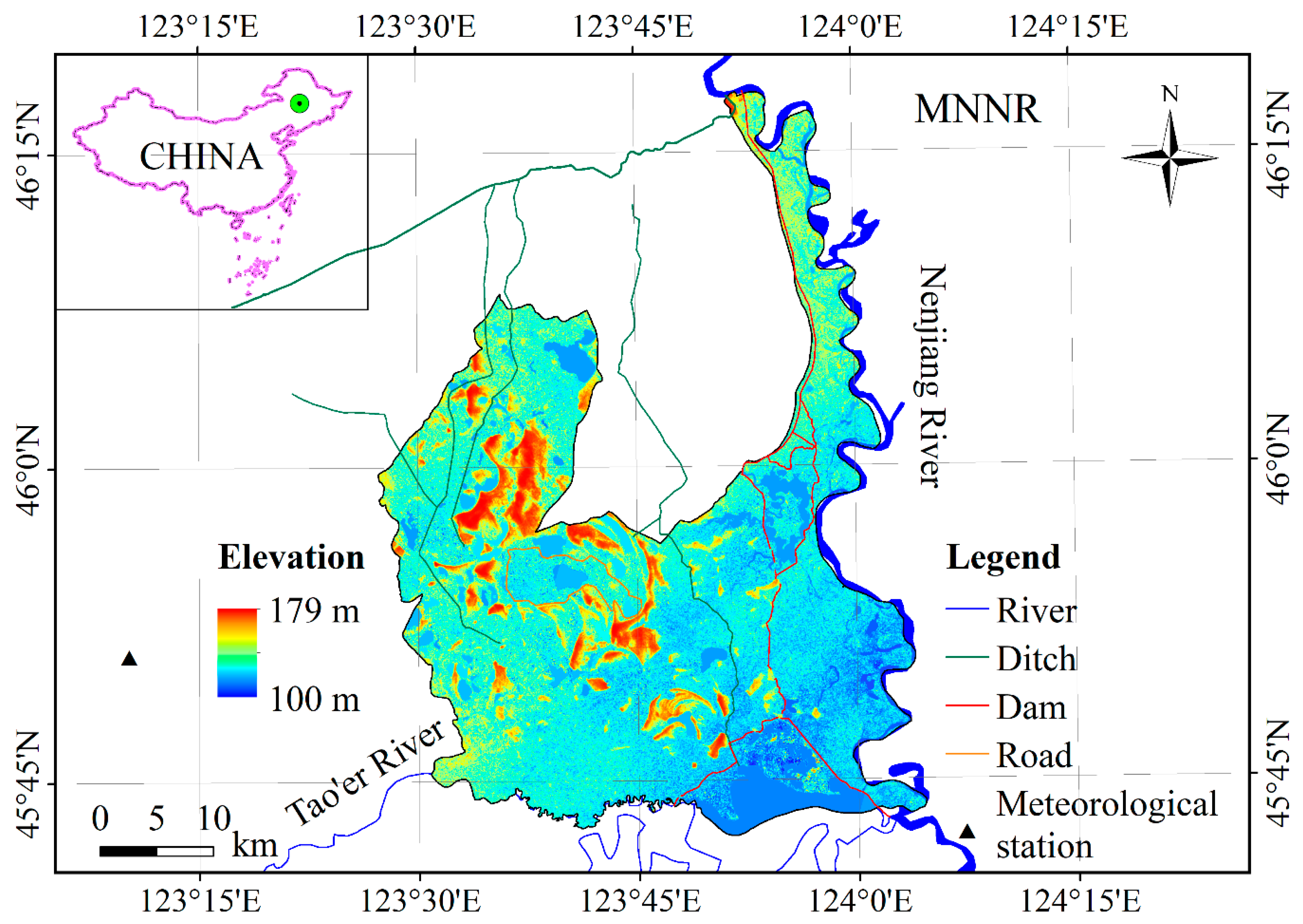
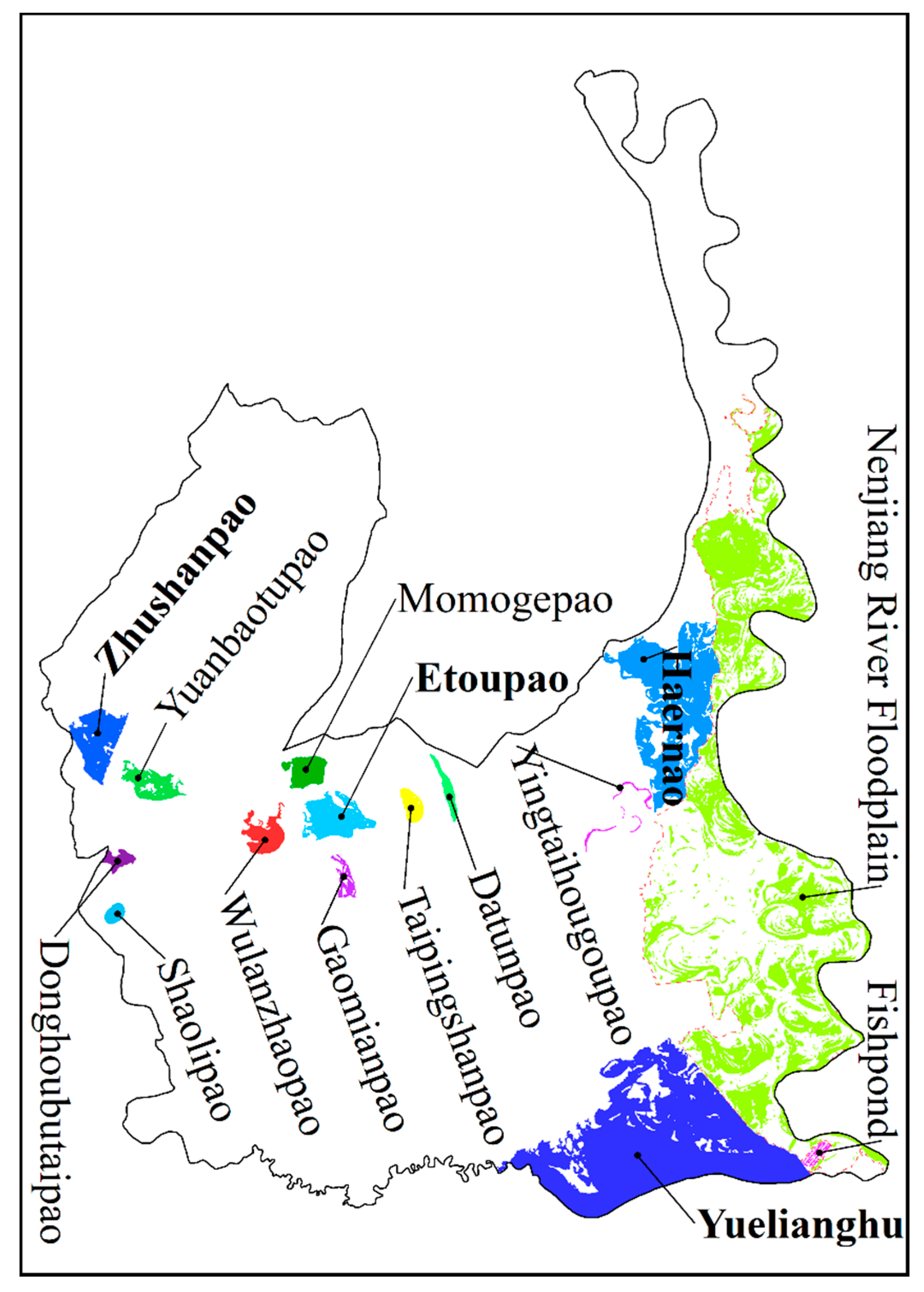
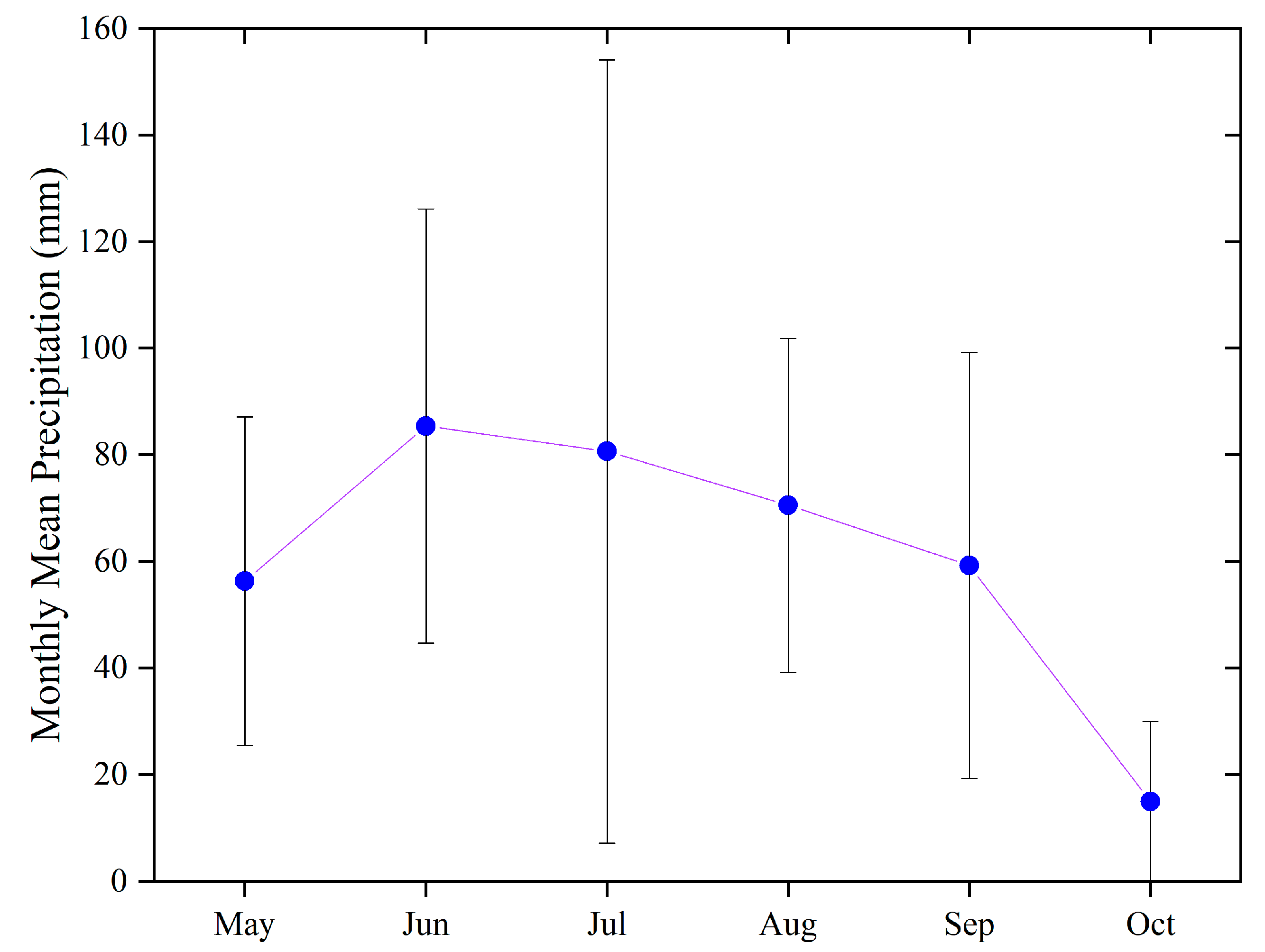
2.1. Study Area

The Momoge National Nature Reserve (45°42′25′′–46°18′00′′ N, 123°27′00′′–124°04′33.7′′ E) covering an area of 1440 km2 is located in Zhenlai County, west Jilin Province, Northeast China (Figure 1). The reserve is known as the main stopover site for rare and endangered migratory birds, such as the Siberian crane (Grus leucogeranus) and oriental white stork (Ciconia ciconia) and was included on the List of Wetlands of International Importance (Ramsar sites) in 2013 [28]. Two large rivers flow through the reserve, the Nenjiang River in the east and the Tao’er River in the south. The reserve has many permanent water bodies including four major open water bodies, the Yuelianghu Reservoir, Haernao Reservoir, Etoupao Lake, and Zhushanpao Lake (Figure 2). The peripheral road of the Etoupao Lake and Wulanzhaopao Lake hindered the connection between these two lakes and the surrounding lakes.
There is also a large dam to the east of the Nenjiang River floodplain, which hinders the hydrological connection between the Nenjiang River and the wetlands to the east of the dam (Figure 1).
Elevation of the MNNR is higher in the northwest and lower in the southeast, with a relative elevation difference of only 2–10 m. The region has a temperate continental monsoon climate with an annual average temperature of 4.97 °C, an annual precipitation of 385.69 mm, and an annual evapotranspiration of 1530.13 mm, respectively [31]. The annual freezing period starts in October, and the annual thawing period is in May. Approximately 90% of the annual precipitation occur from May to October. Figure 3 shows the mean monthly precipitation from May to October in the study area in recent years (2015–2019).
Since the continuous dry years since the 1990s, the amount of natural recharging water in the reserve has been decreasing, which is 70% lower than that in the late 1950s and early 1960s [32]. To adapt to this climate change, various water conservancy facilities such as reservoirs, dams, and ditches have been built upstream of the MNNR. However, these human activities have led to a serious decline in the hydrological connectivity of the reserve, which in turn poses a serious threat to the health of wetland ecosystems. In recent years, local managers have carried out ecological replenishment to the wetlands by dispatching the water from the Nenjiang River and farmland discharge through irrigation and drainage ditch networks (Figure 1).

2.2. Methodology

2.2.1. SAR Data Collection

Surface water dynamics were derived from a time series of Sentinel-1 Ground Range Detected (GRD) scenes acquired between 2015 to 2019. Google Earth Engine (Google, Inc., Mountain View, CA, USA) has pre-processed the GRD products into backscatter coefficients (σ°) imagery in decibels (dB). The pre-processing steps include applying orbit file, removing GRD border noise, removing thermal noise, radiometric calibration, and terrain correction (orthorectification). A total of 235 Sentinel-1 C-VV backscatter coefficient products with a spatial resolution of 10 × 10 m was downloaded from Google Earth Engine. However, scenes from the late October to early May were excluded from the analysis because ice could be seen on the lakes, which inhibited the SWE extraction. Table 1 enumerates the 52 images finally used in this study.

2.2.2. SAR Data Processing and Wet and Dry Binary State Data Generation

In order to minimize the influence of salt-and-pepper noise on the SWE retrieval, a Median filter with a kernel of 9 × 9 pixels was applied to the backscatter coefficient data. The Median filter replaces each center pixel with the median value within the neighborhood specified by the filter size. Afterwards, we applied the “Minimum Error” automatic threshold method [33] to the filtered grayscale imagery to creat a new series of raster (i.e., wet and dry binary state data), where the values below the specified threshold are set to 1 (denotes wet pixels) and all other values are set to 0 (denotes dry pixels). This method approximates the histogram as a bimodal Gaussian distribution and finds a cut-off point. The cost function is based on the Bayes classification rule [33]. Subsequently, a stratified random sampling method was used to select a total of 200 points from Google Earth historical images to evaluate the overall accuracy of the derived wet and dry binary state rasters. The ENVI software (version 5.5.3, Harris Geospatial Solutions, Inc., Broomfield, CO, USA) was used for the above processing.

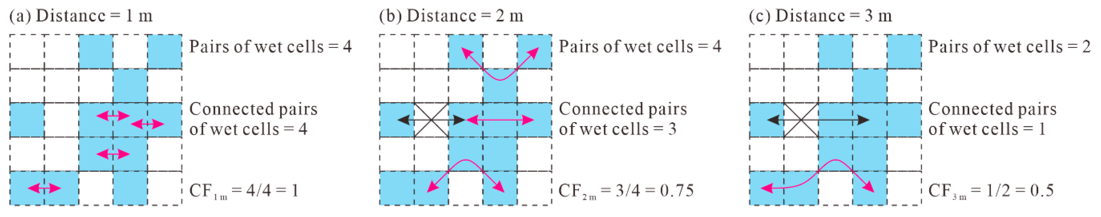
2.2.3. Geostatistical Connectivity Function

The GCF was used in this study to assess the magnitude and extent of surface water connections. The GCF represents the probability that n pixels along a given direction are all valued higher than the threshold z c [34]:
P ( n ; z c ) = Pr { j = 1 n I ( u j ; z c ) = 1 }
where Π is the product operator. I ( u j ; z c ) is an indicator of the z ( u j ) at location u j that above the threshold value z c , defined as I ( u j ; z c ) = 1 if z ( u j ) > z c , zero if not. It is estimated when the starting wet pixel u 1 takes all possible positions within the wet and dry binary state data. Therefore, the value of the GCF at any given distance is the proportion of pairs of connected wet pixels in pairs of total (i.e., connected and isolated) wet pixels along a given direction.
The surface water connectivity analysis applied in this study is based on a MATLAB (The MathWorks, Inc., Natick, MA, USA) scriptprovided by Trigg et al. [29]. The MATLAB program analysises on wet and dry binary state data and calculates the GCF in four directions, i.e., West–East (W–E), North–South (N–S), Northwest–Southeast (NW–SE) and Northeast–Southwest (NE–SW). A simple example shows how to calculate the GCF in the W–E direction, assuming 8-way connectivity (Figure 4). Besides, the program outputs a grid in which each connectome is identified by an integer number ranging from 1 to n. On this basis, we identify the top ten largest connectomes and the remaining connected/isolated water bodies. The MATLAB software (version R2014a)and the ArcGis software (version 10.7, Environmental Systems Research Institute, Redlands, CA, USA) were used for the above processing.

2.2.4. Connection Frequency Analysis

The surface water connectivity within the MNNR were further assessed by an index called “connection frequency” [20]:
Fcon = Ncon/Ntot
where Fcon is the connection frequency (%), Ncon is the total number of incidents of surface water connectivity, and Ntot is the total number of images. The ArcGis software (version 10.7, Environmental Systems Research Institute, Redlands, CA, USA) was used for the above processing.

2.2.5. Statistical Analysis

A one factor analysis of variance (ANOVA) was performed to determine whether there were significant differences in connection frequency in different months. If significant differences were revealed, Dunnett’s T3 tests (p ≤ 0.01) were used for the separation of means. The statistical procedures were conducted by SPSS software (Version 25, SPSS, Chicago, IL, USA).

3. Results

3.1. Changes in the GCF

The overall accuracy of the wet and dry binary state (i.e., water and non-water) rasters derived from Sentinel-1 A/B GRD products ranges from 95.72% to 98.15%. Based on the wet and dry binary state rasters, the application of the geostatstical connectivity analysis creates a series of CF curves that reflect the ever-changing surface water connectivity from May to October during normal years. For clarity, this is illustrated in four direcitons (i.e., W–E, N–S, NW–SE and NE–SW) in Figure 5, Figure 6, Figure 7 and Figure 8.

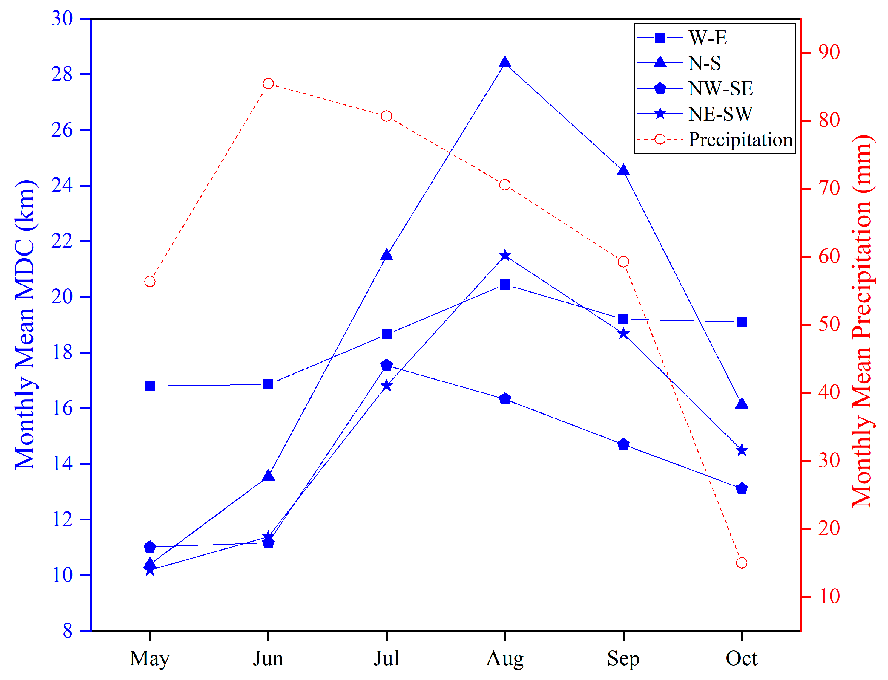
3.1.1. Changes in the GCF in the W–E Direction

The GCF curve in the W–E direction drops rapidly in all months and eventually reaches zero (Figure 5). The maximum distance of connection (MDC, i.e., the distance at which the GCF curve reaches zero) was 16.80 (std: ±1.00) km in May, 16.85 (±1.74) km in June, 18.66 (±2.42) km in July, 20.45 (±3.67) km in August, 19.20 (±2.89) km in September and 19.09 (±3.73) km in October, respectively (Figure 5). The general trend of MDC in the W–E direction is to change little from May to June, then increase moderately from June to August, and then decrease slowly from August to October (Figure 5g).

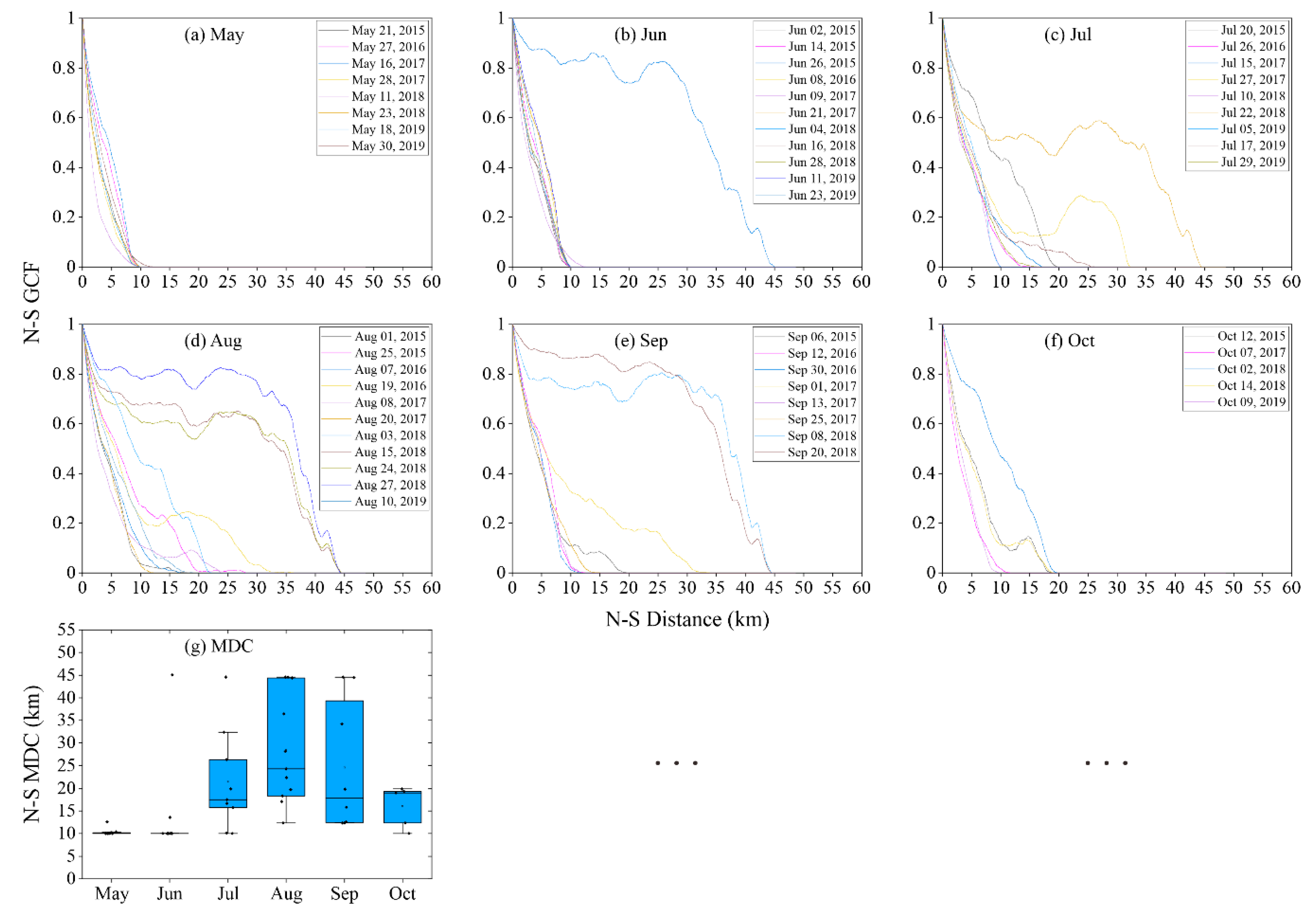
3.1.2. Changes in the GCF in the N–S Direction

Unlike the W–E direction, the GCF curve in the N–S direction drops sharply in May, June, and October, while it decreases slowly in July, August, and September (Figure 6). The MDC was 10.39 (±0.89) km in May, 13.55 (±10.49) km in June, 21.47 (±11.22) km in July, 28.39 (±12.06) km in August, 24.52 (±14.28) km in September and 16.13 (±4.57) km in October, respectively (Figure 6). The general trend of MDC in the N–S direction is to increase moderately from May to June, then rise sharply from June to August, and then decline sharply from August to October (Figure 6g).

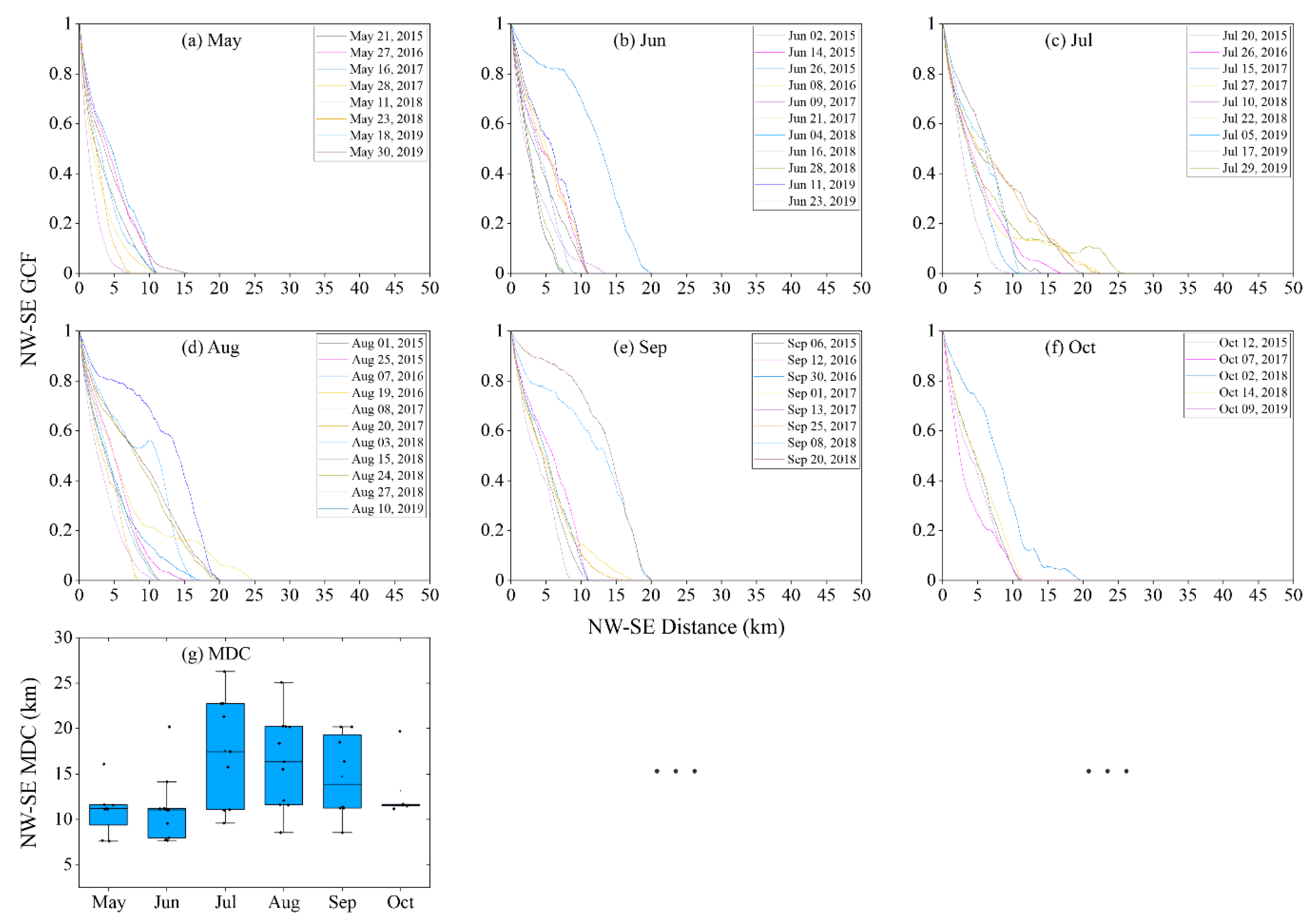
3.1.3. Changes in the GCF in the NW–SE Direction

The GCF curve of each month decline more sharply in the NW–SE direction than in the W–E direction, and eventually becomes zero (Figure 7). The MDC was 11.01 (±2.65) km in May, 11.17 (±3.56) km in June, 17.54 (±6.08) km in July, 16.33 (±4.99 km in August, 14.70 (±4.62 km in September and 13.12 (±3.67) km in October, respectively (Figure 7). The general trend of MDC in the NW–SE direction is to change little from May to June first, then rise a lot from June to July, and decline gradually from July to October (Figure 7g).

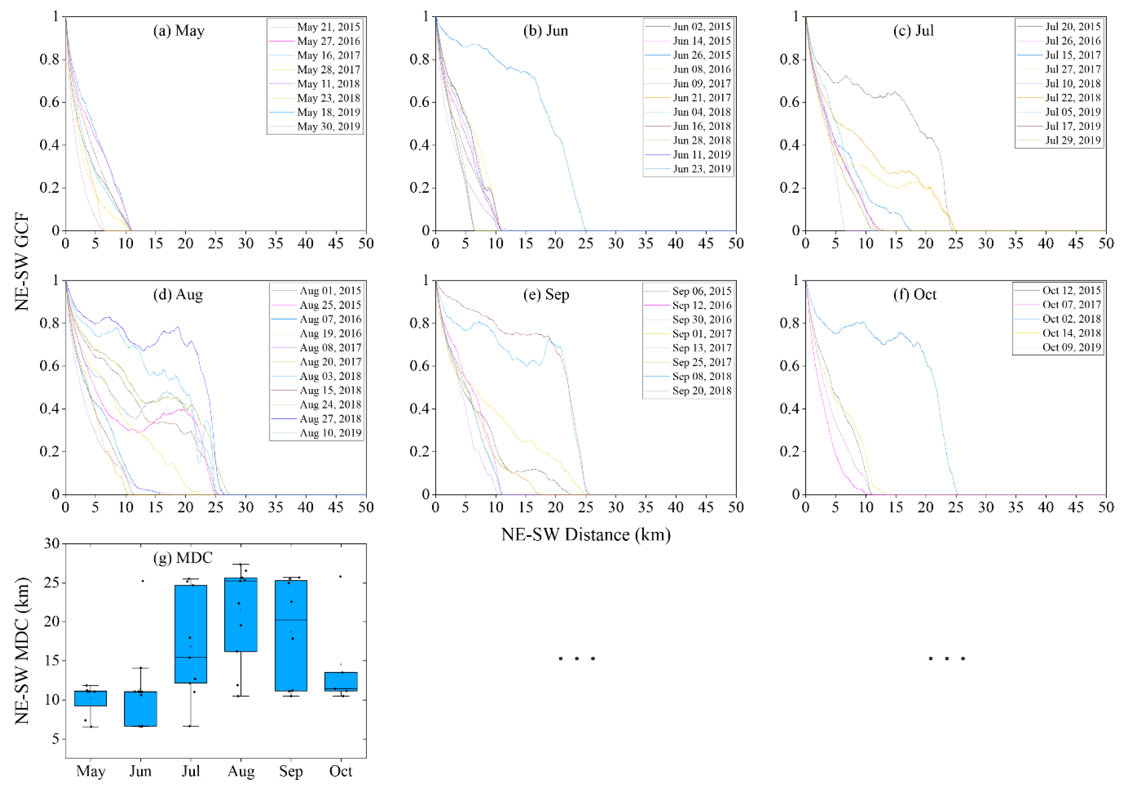
3.1.4. Changes in the GCF in the NE–SW Direction

Although the trend is similar, the monthly downward trend of the GCF curve in the NE–SW direction is greater than that in the N–S direction (Figure 8). The MDC was 10.19 (±2.00) km in May, 11.38 (±5.17) km in June, 16.81 (±6.95) km in July, 21.49 (±6.07) km in August, 18.68 (±6.87) km in September and 14.49 (±6.43) km in October, respectively (Figure 8). The general trend of MDC in the NE–SW direction is to increase slightly from May to June first, then rise a lot from June to August, and decline gradually from August to October (Figure 8g).

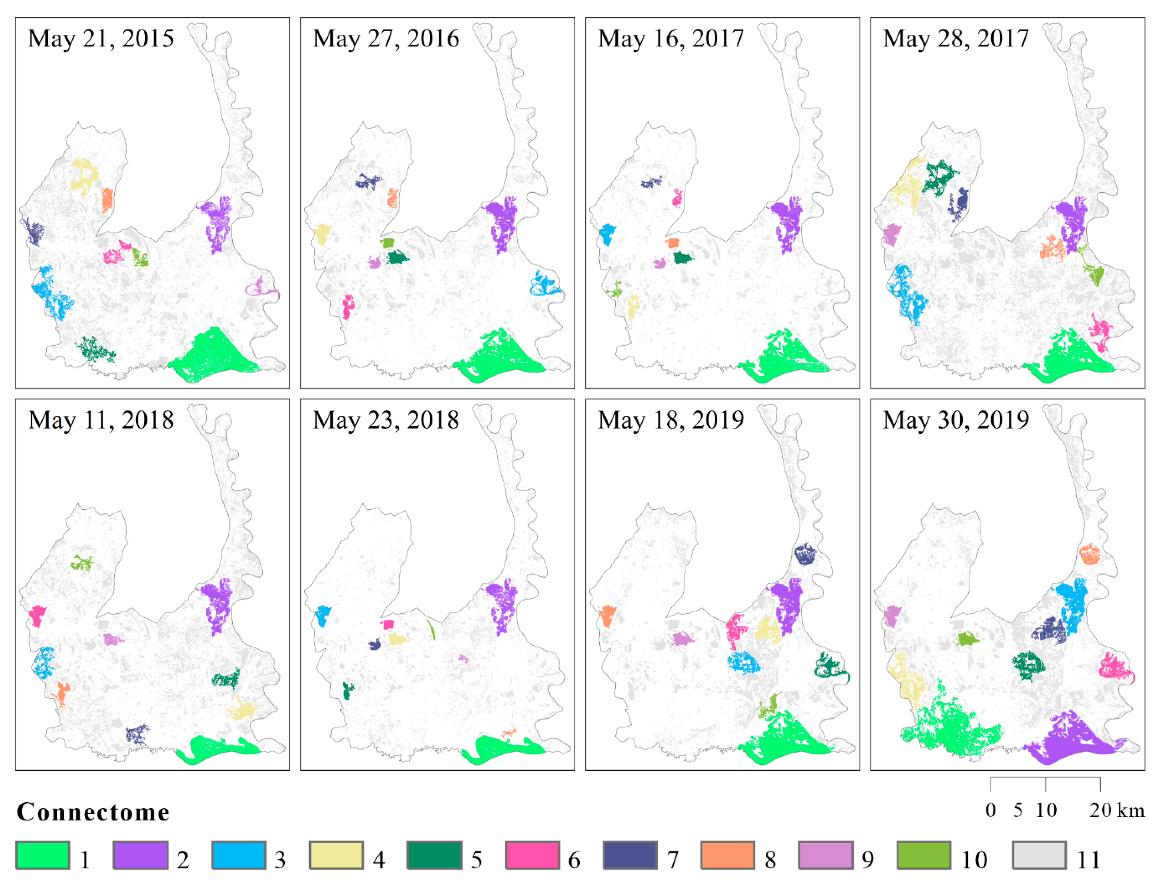
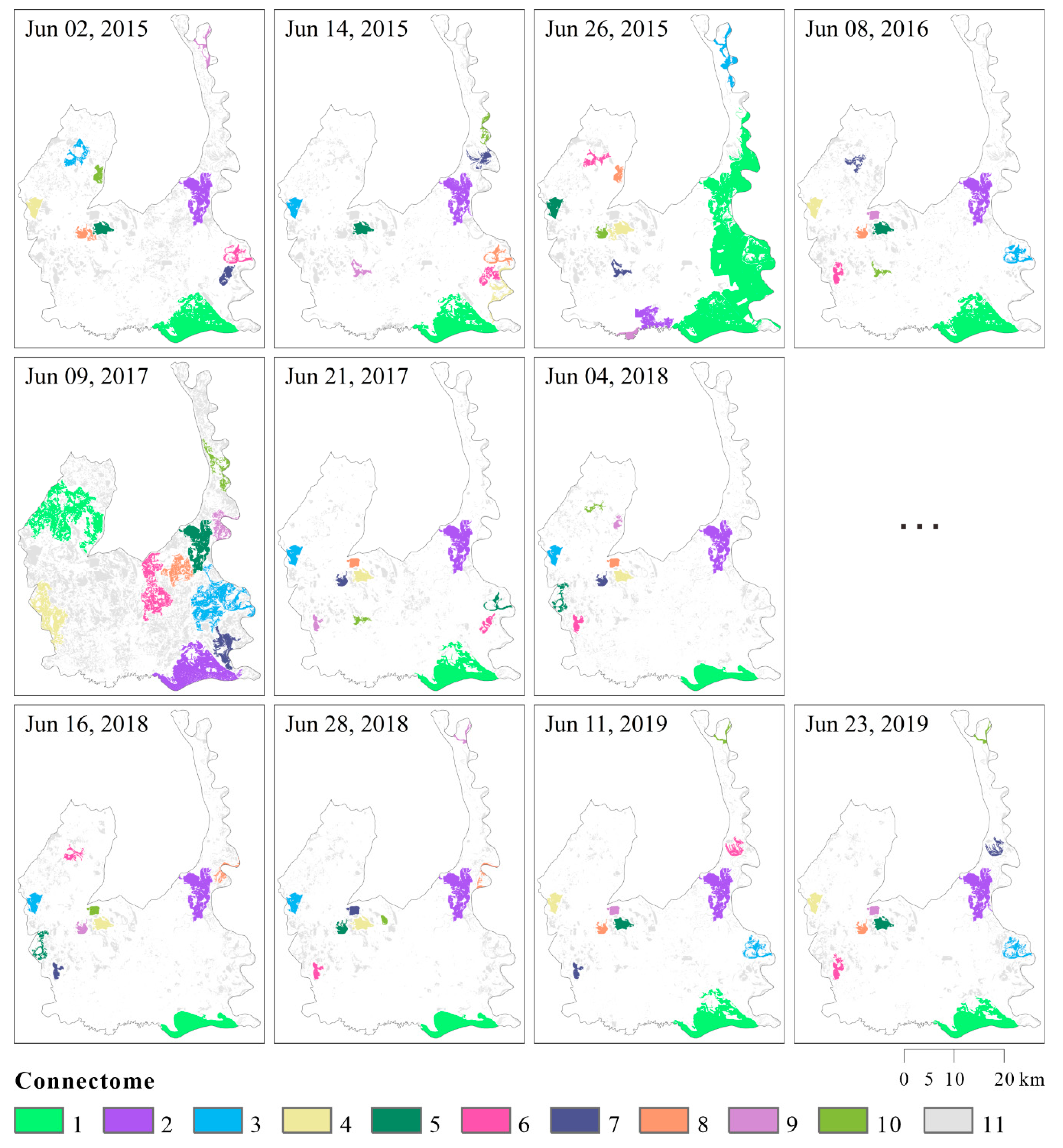
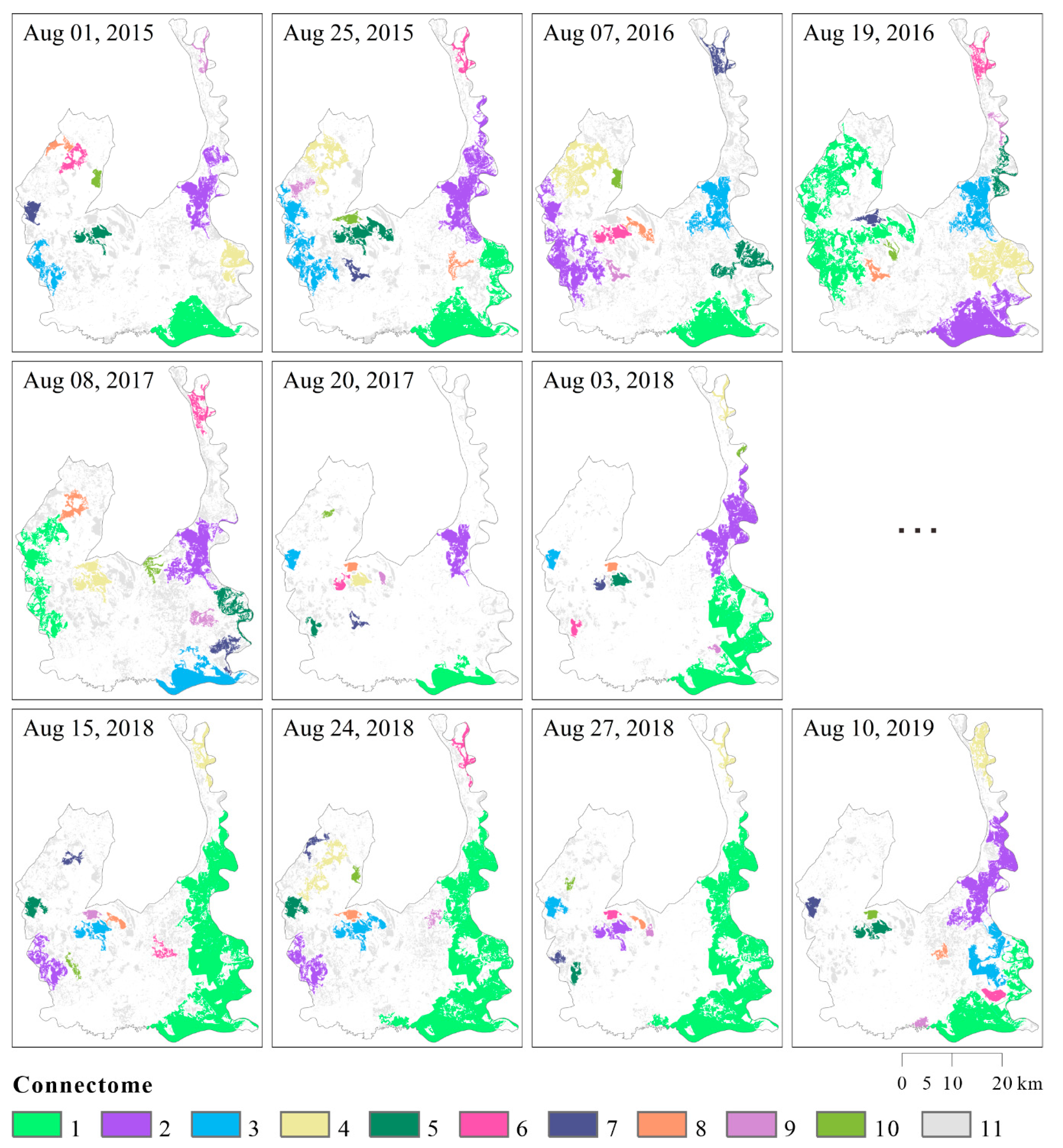
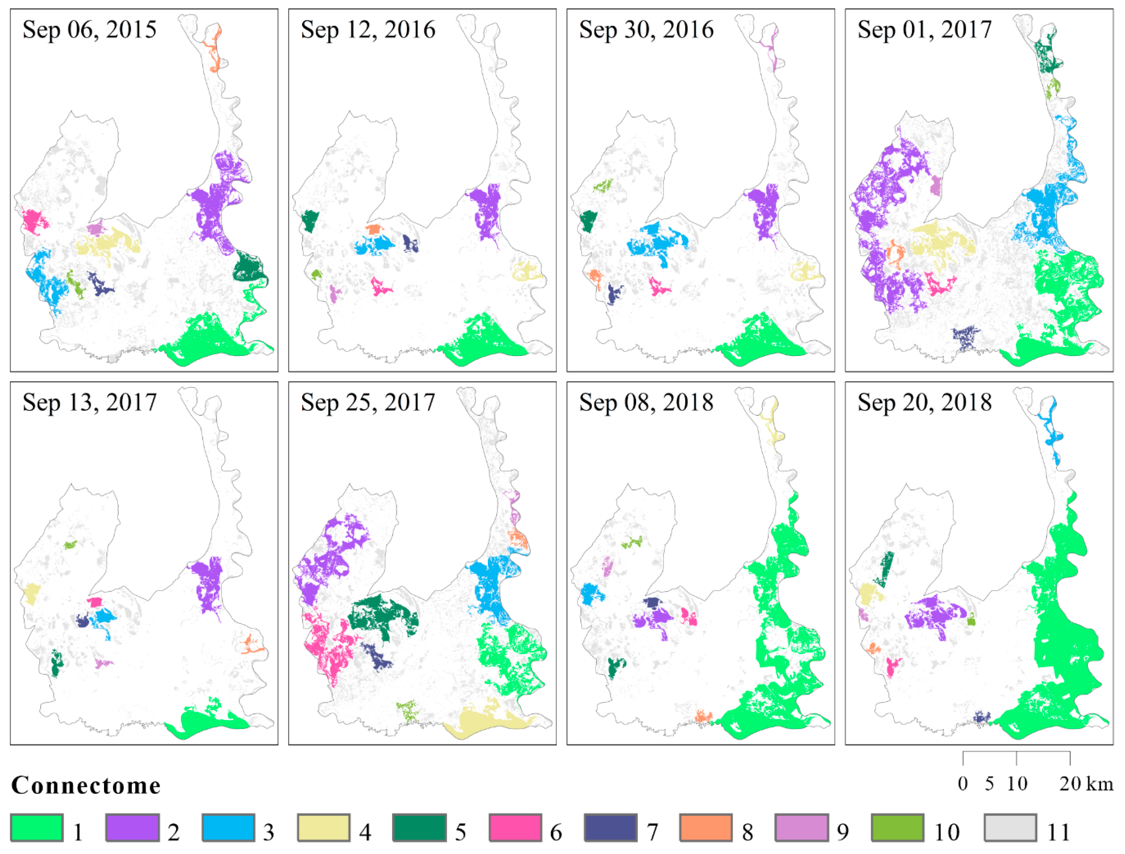
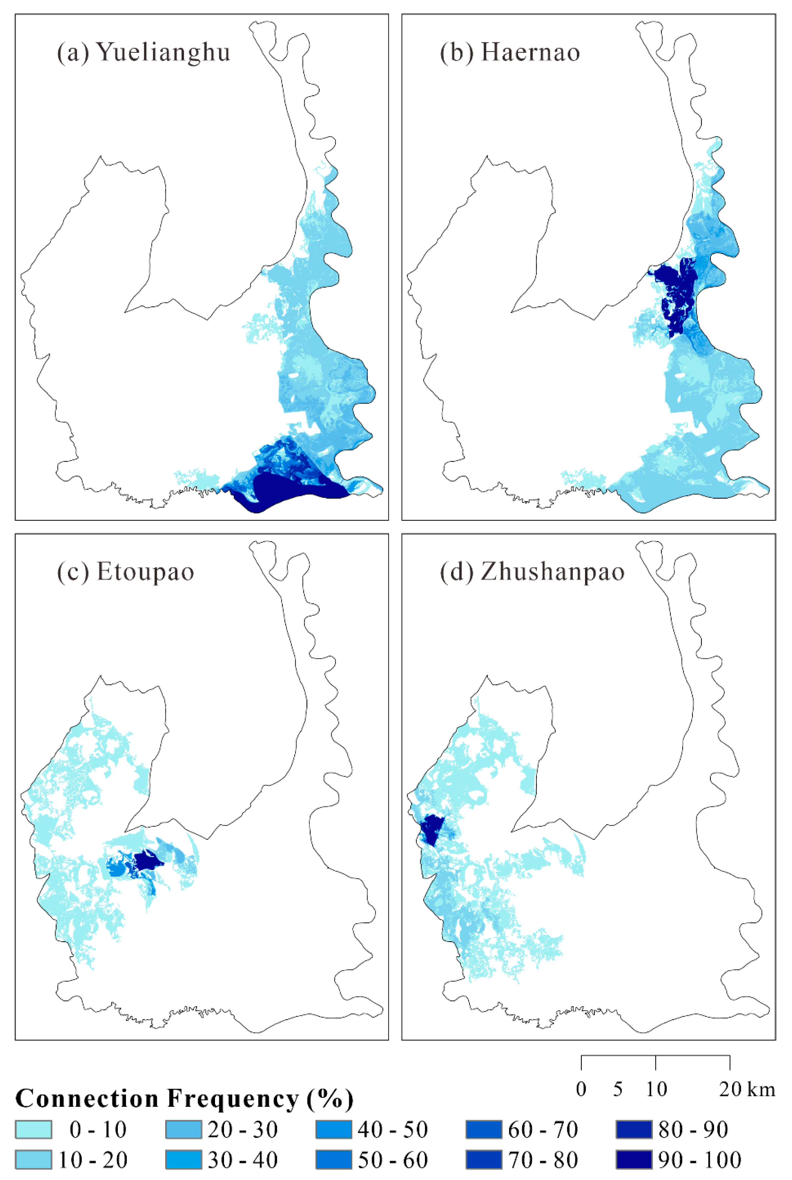
3.2. Spatial-Temporal Distribution and Connection Process of the Main Connectomes

There are four largest permanent water bodies in the study area, namely Yuelianghu in the southeast, Haernao in the northeast, Etoupao in the north-central and Zhushanpao in the west (Figure 2). The four largest permanent water bodies are frequently connected to the surrounding lakes, thus forming the four main connectomes. Figure 9, Figure 10, Figure 11, Figure 12, Figure 13 and Figure 14 depict the spatial-temporal distribution of the connectomes in MNNR.
As seen, except for the occasional connection between the Yuelianghu and the fishpond, most water bodies were isolated from each other in May. In June, the Yueliagnhu and the fishpond still occasionally connect with each other, and there was also an occasional connection between the Yueliagnhu and the the Nenjiang River floodplain. Meanwhile, the Haernao began to occasionally connect with three water bodies (i.e., the Nenjiang River floodplain, the Yuelianghu and the fishpond) via floodplain channels and diffusive overbank flow. In July, the connections between several pairs of water bodies (i.e., the Yuelianghu and the fishpond, the Yuelianghu and the Nenjiang River floodplain, the Harnao and the Nenjiang River floodplain) became frequent. Meanwhile, the Haernao began to frequently connect with the Yingtaihougoupao through a sluice gate. Inaddition, the water bodies in the eastern part of MNNR (i.e., the Yuelianghu, the fishpond, the Nenjiang River floodplain, the Harnao and the Yingtaihougoupao) occasionally connected to each other, forming one single water body. Due to “fill-and-spill” and “fill-and-merge”, the Etoupao began to connect frequently with the Wulanzhaopao via a channel. Meanwhile, as the water overflowed from the peripheral road, the Etoupao began to be frequently connected to the Gaomianpao and occasionally to the Taipingshanpao. At the same time, the Zhushanpao was occasionally connected with several lakes (i.e., the Yuanbaotupao, the Donghoubutaipao and the Shaolipao) through overflow. In August, there was an occasional connection between the Etoupao and the Momogepao via the over-road flow. During this period, the Zhushanpao and the Yuanbaotupao were isolated from each other. Meanwhile, the lakes in the north-central and western parts of the MNNR (i.e., the Zhushanpao, the Wulanzhaopao, the Etoupao, the Taipingshanpao, the Datunpao, the Donghoubutaipao and the Shaolipao) were occasionally connected to each other to form a single water body. In addition, the connection frequency between other lakes in August was about the same as in July. In September, the connection between the Etoupao and two lakes (i.e., the Taipingshanpao and the Momogepao) became frequent. During this period, the Zhushanpao and the Shaolipao were isolated from each other, and the Etoupao connectome in the north-central MNNR and the Zhushanpao connectome in the west MNNR were also isolated from each other. Besides, the connection frequency between other lakes in September was almost the same as in August. In October, most water bodies were isolated from each other, and the connection frequency of two pairs of lakes (i.e., the Etoupao and the Taipingshanpao, the Etoupao and the Wulanzhaopao) reduced. However, three pairs of water bodies (i.e., the Yuelianghu and the Nenjiang River floodplain, the Haernao and the Nenjiang River floodplain, as well as the Etoupao and the Gaomianpao) were still frequently connected.

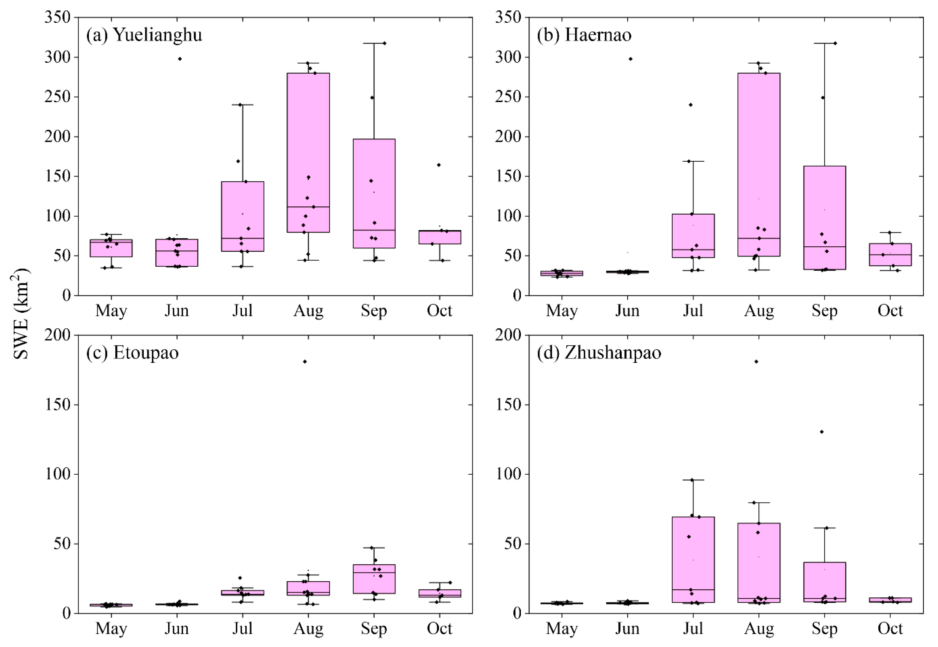
3.3. Variations in SWE of the Main Connectomes

The extent of the four main connectomes changed throughout the study period, and their variations were smallest in the spring and highest in the summer months.
The SWE of the Yuelianghu connectome was 60.62 (±16.15) km2 in May, 76.36 (±74.61) km2 in June, 102.46 (±67.50) km2 in July, 146.03 (±94.68) km2 in August, 129.86 (±101.32) km2 in September, and 87.34 (±45.77) km2 in October (Figure 15a). The general trend of the SWE of the Yuelianghu connectome is that it rises slowly from May to June, rises rapidly from June to August, and falls rapidly from August to October.
The SWE of the Haernao connectome was 27.82 (±3.24) km2 in May, 54.24 (±80.82) km2 in June, 88.02 (±71.57) km2 in July, 121.35 (±106.97) km2 in August, 108.04 (±110.99) km2 in September and 53.12 (±19.70) km2 in October, respectively (Figure 15b). The general trend of the SWE of the Haernao connectome is that it rises slowly from May to June, rises rapidly from June to August, and falls rapidly from August to October.
The SWE of the Etoupao connectome was 6.06 (±0.83) km2 in May, 6.71 (±0.79) km2 in June, 14.72 (±5.29) km2 in July, 30.94 (±50.18) km2 in August, 26.86 (±12.97) km2 in September and 14.41 (±5.37) km2 in October, respectively (Figure 15c). The general trend of the SWE of the Etoupao connectome is that it maintains the level from May to June, rises slowly from June to August, and falls slowly from August to October.
The SWE of the Zhushanpao connectome was 7.41 (±0.56) km2 in May, 7.65 (±0.66) km2 in June, 38.27 (±34.32) km2 in July, 40.65 (±53.88) km2 in August, 31.32 (±44.02) km2 in September and 9.41 (±1.65) km2 in October, respectively (Figure 15d). The general trend of the SWE of the Zhushanpao connectome is that it maintains the level from May to June, rises rapidly from June to July, rises slowly from July to August, and falls gradually from August to October.

3.4. Connection Frequency of the Main Connectomes

In terms of time, at the 0.01 significance level, the monthly mean connection frequency in August was significantly higher than that in May and June. However, no significant differences in the monthly mean connection frequency among the other months were found (Table 2).
Spatially, for the Yuelianghu connectome, the connection frequency was 51.9% between the Yuelianghu and the Nenjiang River floodplain, 48.1% between the Yuelianghu and the fishpond, 15.4% between the Yuelianghu and the Haernao, and 9.6% between the Yuelianghu and the Yingtaihougoupao, respectively (Figure 16a). For the Haernao connectome, the connection frequency was 55.8% between the Haernao and the Nenjiang River floodplain, 32.7% between the Haernao and the Yingtaihougoupao, 15.4% between the Haernao and the Yuelianghu, and 15.4% between the Haernao and the fishpond, respectively (Figure 16b). For the Etoupao connectome, the connection frequency was 48.1% between the Etoupao and the Wulanzhaopao, 40.4% between the Etoupao and the Gaomianpao, 21.2% between the Etoupao and the Taipingshanpao, 9.6% between the Etoupao and the Momogepao, 1.9% between the Etoupao and the datunpao, 1.9% between the Etoupao and the west lakes (i.e., the Zhushanpao, the Donghoubutaipao, and the Shaolipao), respectively (Figure 16c).
For the Zhushanpao connectome, the connection frequency was 15.4% between the Zhushanpao and the Donghoubutaipao, 7.7% between the Zhushanpao and the Shaolipao, 5.7% between the Haernao and the Yuanbaotupao, and 1.9% between the Haernao and the north-central lakes (i.e., the Wulanzhaopao, the Etoupao, the Taipingshanpao and the Datunpao), respectively (Figure 16d).

4. Discussion

Our study shows that two key characteristics of the geostatistical connectivity function can be used to identify important changes in a surface hydrological connectivity system. One is the reduction rate of the GCF, namely, the slower the rate is, the higher the connectivity will be. The other characteristic is the change of maximum distance of connection, i.e., the longer the MDC is, the higher the connectivity will be.
In the present study, as the distance increased, the GCF gradually dropped from 1 (fully connected) to 0 (complete isolation) in all cases (Figure 5, Figure 6, Figure 7 and Figure 8). This is different from the seasonal isolated river-lake system in the China’s Poyang Lake National Nature Reserve (PLNNR) and its vicinity, where the minimum GCF in the W–E direction near the flood peak in a normal year was higher than 0.65 [19], indicating that the surface hydrological connectivity along the W–E direction in this area is better than that in the MNNR. However, the decline rates of the GCF in the four directions in our study indicate that the difference in the magnitude of surface hydrological connection was greater in the N–S and NE–SW directions than in the W–E and NW–SE directions (Figure 5, Figure 6, Figure 7 and Figure 8). This is because the GCF in the N–S and NE–SW directions is mainly controlled by the SWE of the Nenjiang River floodplain, and the SWE of the Nenjiang River floodplain varies greatly in these two directions. When the SWE in the Nenjiang River floodplain reaches its maximum value, the GCF in the N–S and NE–SW directions also reaches the maximum value. However, the SWE of the Nenjiang Plain has little effect on the GCF in the W–E and NW–SE directions. This is due to the barrier effect of the extremely long Nenjiang Dam. Correspondingly, monthly MDC seems to be separated by two important thresholds. In most cases, The MDC along the W–E, NW–SE and NE–SW directions were shorter than 25 km, whereas the MDC along the N–S direction was shorter than 45 km. Similar MDC threshold effects have also been observed in the river-lake system of the China’s Poyang Lake floodplain [19,20] as well as in a river-floodplain system in Bangkok, Thailand [29], although thresholds and their causes are different.
As can be seen from Figure 17, generally, the changes in monthly mean MDC from May to June and from August to October are consistent with the changes in mean monthly precipitation, while from June to August, the two trends are opposite along most of the four directions. This indicates that from June to August, MDC has a lagging effect on precipitation change. One possible explanation for this is that the rainwater received by the lakes has a cumulative effect, with more water stored in the lakes than consumed from June to August, although absolute precipitation has been decreasing during this period.
The time series imagery established by combining geostatistical analysis and remote sensing methods reflect the distribution, flow paths and connection process of the MNNR connectomes (Figure 9, Figure 10, Figure 11, Figure 12, Figure 13 and Figure 14). As can be seen, there are four water bodies (i.e., the Yuelianghu, Haernao, Etoupao and Zhushanpao) that can enter the top ten connectomes list almost every time. This is because all four water bodies are directly and intermittently supplemented with water. However, sometimes some water bodies that are not supplemented with water suddenly appear in the list of the top ten connectomes. The reasons can be divided into two cases according to the location of the water bodies: (i) for water bodies adjacent to the Nenjiang River, it is mainly due to floods of the Nenjiang River; (ii) for water bodies far from the Nenjiang River, it may be due to irregular recharge of groundwater and rainwater. Additionally, when a connectome is formed depends on the hydrological season and the timing of water replenishment, while the flow paths between seasonally isolated lakes vary according to geomorphologic characteristics as well as the distribution of the artificial channels. In short, natural and human factors affect the formation, timing, duration, flow path and scale of the hydrological connection in MNNR. This is similar to a river-lake system in the Poyang Lake floodplains, which is affected by both natural and human factors such as geomorphic features, hydrological years, and human manipulations [19].
It can be seen from Figure 18 that from June to August, the trend of SWE is opposite to the trend of precipitation, which indicates that SWE change during this period also has a lagging effect compared with precipitation change. Among the four main connectomes, the monthly mean SWE of the Yuelianghu connectome was the largest, mainly because the connectomes had the most water sources, including the Nenjiang River, Tao’er River and farmland backwater. The monthly mean SWE of the Haernao connectome was the second largest, mainly due to the water source of the connectome is the Nenjiang River. The monthly mean SWE of the Etoupao and Zhushanpao connectomes was much smaller because they are supplemented mainly by artificial ditches. This implies that the flow of artificial ditches may be much less than that of natural rivers. Our study also shows that the connection frequency between water bodies mainly depends on three factors, including whether they are geographically adjacent, whether they are connected by channels, and whether they are blocked by dams. This finding is consistent with [19]. Moreover, these is also a lagging effect between connection frequency changes and precipitation changes from June to August (Figure 19).
This study demonstrates that the combination of SAR data and geostatistical metrics is well-suited for detecting surface hydrological connectivity in an ungauged area. Compared with using surface water extent and connection frequency alone, the specific advantages of using the geostatistical connection function are that it can help resource managers and decision makers identify changes in surface hydrological connectivity, as well as address potential impacts of these changes on water resources for human use and/or ecological integrity at the landscape level. While we expect that this approach can be applicable to other regions, two limitations should be noted. First, the temporal-spatial resolution of Sentinel-1 SAR data used in this study is still too coarse to detect timing, duration and details of hydrological connectivity, such as the narrow channel that supplies Etoupao. Second, swamp and marsh wetlands may be hydrologically connected to open waters, but it is difficult to identify these wetlands with SAR imageries. However, Canada’s new generation of three identical SAR satellites, the RADARSAT Constellation Mission (RCM), launched in June 2019 provide a repeat cycle of 4 days and a spatial resolution of 5 m. These images are expected to greatly increase spatiotemporal resolution of SAR data, and are expected to solve the first limitation. A solution to the second limitation still needs an advancement in remote sensing interpretation technology. Up to now, it is not only challenging to identify swamp and marsh wetlands using SAR data, but also difficult to quickly and accurately identify these wetlands with optical data in general.

5. Conclusions

The surface hydrological connectivity dynamics for a multi-lake system, China’s Momoge National Nature Reserve, a Ramsar recognized wetland site of international importance, has been quantified using a geostatistical method applied to a Sentinel-1 SAR product. We found that the geospatial connectivity function (GCF), maximum distance connection (MDC), and surface water extent (SWE) derived from this approach changed continually throughout the 5-year study period from 2015 through 2019. The difference in the GCF was greater in the N–S and NE–SW directions than in the W–E and NW–SE directions due to the barrier effect of a north-south river dam. The MDC showed a threshold effect, generally less than 25 km in the W–E, NW–SE and NE–SW directions, and less than 45 km in the N–S direction. In general, monthly means of MDC, SWE and connection frequency all increased from May to August, but decreased from August to October. The trend of these indicators from June to August were opposite to mean monthly precipitation, which may be due to the amount of water stored in the water bodies exceeding the amount of water consumed during these months. Our results also revealed that water supply sources, obstacles and geographical distance were the main factors affecting the surface hydrological connectivity of the study area. The use of geostatistical connectivity function metrics combined with Sentinel-1 SAR data allowed us to investigate the dynamics of surface hydrological connectivity without being affected by clouds. The study demonstrates the usefulness of the geostatistical method combining Sentinel-1 SAR image analysis in quantifying surface hydrological connectivity in an ungagged area. This approach should be applicable for other geographical regions, in order help resource managers identify whether and how to change the status of surface hydrological connectivity, as well as address potential impacts of these changes on water resources for human use and/or ecological integrity at the landscape level.

Author Contributions

Conceptualization, Y.C., L.W. and G.Z.; methodology, Y.C., L.W. and Y.J.X.; software, Y.C. and Z.T.; validation, G.Z., Y.C. and L.W.; formal analysis, Y.C. and L.W.; investigation, S.Q.; data curation, Y.C.; writing—original draft preparation, Y.C.; writing—review and editing, Y.J.X., G.Z. and Y.C. All authors have read and agreed to the published version of the manuscript.

Funding

This research was funded by the National Natural Science Foundation of China (41701395, 41877160); the National Key R & D Program of China (2017YFC0406003); the Nanhu Scholars Program for Young Scholars of XYNU; and the U.S. Department of Agriculture Hatch Fund project (LAB94459).

Conflicts of Interest

The authors declare no conflict of interest.

References

  1. Ward, J.V. The four-dimensional nature of lotic ecosystems. J. N. Am. Benthol. Soc. 1989, 8, 2–8. [Google Scholar] [CrossRef]
  2. Bracken, L.J.; Croke, J. The concept of hydrological connectivity and its contribution to understanding runoff-dominated geomorphic systems. Hydrol. Process. 2007, 21, 1749–1763. [Google Scholar] [CrossRef]
  3. Fritz, K.M.; Schofield, K.A.; Alexander, L.C.; Mcmanus, M.G.; Golden, H.E.; Lane, C.R.; Kepner, W.G.; Leduc, S.D.; Demeester, J.E.; Pollard, A.I. Physical and chemical connectivity of streams and riparian wetlands to downstream waters: A synthesis. J. Am. Water Resour. Assoc. 2018, 54, 323–345. [Google Scholar] [PubMed]
  4. Pringle, C. What is hydrologic connectivity and why is it ecologically important? Hydrol. Process. 2003, 17, 2685–2689. [Google Scholar] [CrossRef]
  5. Saco, P.M.; Rodríguez, J.F.; Moreno-de las Heras, M.; Keesstra, S.; Azadi, S.; Sandi, S.; Baartman, J.; Rodrigo-Comino, J.; Rossi, M.J. Using hydrological connectivity to detect transitions and degradation thresholds: Applications to dryland systems. Catena 2020, 186, 104354. [Google Scholar] [CrossRef]
  6. Leibowitz, S.G.; Wigington, P.J., Jr.; Schofield, K.A.; Alexander, L.C.; Vanderhoof, M.K.; Golden, H.E. Connectivity of streams and wetlands to downstream waters: An integrated systems framework. J. Am. Water Resour. Assoc. 2018, 54, 298–322. [Google Scholar] [PubMed]
  7. Leibowitz, S.G.; Mushet, D.M.; Newton, W.E. Intermittent surface water connectivity: Fill and spill vs. Fill and merge dynamics. Wetlands 2016, 36, S323–S342. [Google Scholar] [CrossRef]
  8. McDonough, O.T.; Lang, M.W.; Hosen, J.D.; Palmer, M.A. Surface hydrologic connectivity between Delmarva Bay wetlands and nearby streams along a gradient of agricultural alteration. Wetlands 2015, 35, 41–53. [Google Scholar] [CrossRef]
  9. Epting, S.M.; Hosen, J.D.; Alexander, L.C.; Lang, M.W.; Armstrong, A.W.; Palmer, M.A. Landscape metrics as predictors of hydrologic connectivity between coastal plain forested wetlands and streams. Hydrol. Process. 2018, 32, 516–532. [Google Scholar] [CrossRef] [Green Version]
  10. Vanderhoof, M.K.; Distler, H.E.; Lang, M.W.; Alexander, L.C. The influence of data characteristics on detecting wetland/stream surface-water connections in the Delmarva Peninsula, Maryland and Delaware. Wetl. Ecol. Manag. 2018, 26, 63–86. [Google Scholar] [CrossRef]
  11. Weiler, M.; McDonnell, J. Virtual experiments: A new approach for improving process conceptualization in hillslope hydrology. J. Hydrol. 2004, 285, 3–18. [Google Scholar] [CrossRef] [Green Version]
  12. Evenson, G.R.; Golden, H.E.; Lane, C.R.; McLaughlin, D.L.; D’Amico, E. Depressional wetlands affect watershed hydrological, biogeochemical, and ecological functions. Ecol. Appl. 2018, 28, 953–966. [Google Scholar] [CrossRef] [PubMed]
  13. Higgisson, W.; Higgisson, B.; Powell, M.; Driver, P.; Dyer, F. Impacts of water resource development on hydrological connectivity of different floodplain habitats in a highly variable system. River Res. Appl. 2020, 36, 542–552. [Google Scholar] [CrossRef]
  14. Golden, H.E.; Lane, C.R.; Amatya, D.M.; Bandilla, K.W.; Kiperwas, H.R.; Knightes, C.D.; Ssegane, H. Hydrologic connectivity between geographically isolated wetlands and surface water systems: A review of select modeling methods. Environ. Model. Softw. 2014, 53, 190–206. [Google Scholar] [CrossRef]
  15. Jones, C.N.; Ameli, A.; Neff, B.P.; Evenson, G.R.; McLaughlin, D.L.; Golden, H.E.; Lane, C.R. Modeling connectivity of non-floodplain wetlands: Insights, approaches, and recommendations. JAWRA J. Am. Water Resour. Assoc. 2019, 55, 559–577. [Google Scholar] [CrossRef]
  16. Beven, K. A manifesto for the equifinality thesis. J. Hydrol. 2006, 320, 18–36. [Google Scholar] [CrossRef] [Green Version]
  17. Golden, H.E.; Creed, I.F.; Ali, G.; Basu, N.B.; Neff, B.P.; Rains, M.C.; McLaughlin, D.L.; Alexander, L.C.; Ameli, A.A.; Christensen, J.R.; et al. Integrating geographically isolated wetlands into land management decisions. Front. Ecol. Environ. 2017, 15, 319–327. [Google Scholar] [CrossRef]
  18. Vanderhoof, M.K.; Alexander, L.C. The role of lake expansion in altering the wetland landscape of the Prairie Pothole Region, United States. Wetlands 2016, 36, S309–S321. [Google Scholar] [CrossRef] [Green Version]
  19. Tan, Z.; Wang, X.; Chen, B.; Liu, X.; Zhang, Q. Surface water connectivity of seasonal isolated lakes in a dynamic lake-floodplain system. J. Hydrol. 2019, 579, 124154. [Google Scholar] [CrossRef]
  20. Liu, X.; Zhang, Q.; Li, Y.; Tan, Z.; Werner, A.D. Satellite image-based investigation of the seasonal variations in the hydrological connectivity of a large floodplain (Poyang Lake, China). J. Hydrol. 2020, 585, 124810. [Google Scholar] [CrossRef]
  21. Huang, S.; Young, C.; Feng, M.; Heidemann, K.; Cushing, M.; Mushet, D.M.; Liu, S. Demonstration of a conceptual model for using LiDAR to improve the estimation of floodwater mitigation potential of Prairie Pothole Region wetlands. J. Hydrol. 2011, 405, 417–426. [Google Scholar] [CrossRef] [Green Version]
  22. White, D.C.; Lewis, M.M. A new approach to monitoring spatial distribution and dynamics of wetlands and associated flows of Australian Great Artesian Basin springs using QuickBird satellite imagery. J. Hydrol. 2011, 408, 140–152. [Google Scholar] [CrossRef] [Green Version]
  23. Whiteside, T.G.; Bartolo, R.E. Use of WorldView-2 time series to establish a wetland monitoring program for potential offsite impacts of mine site rehabilitation. Int. J. Appl. Earth Obs. Geoinf. 2015, 42, 24–37. [Google Scholar] [CrossRef]
  24. Kim, J.-W.; Lu, Z.; Jones, J.W.; Shum, C.K.; Lee, H.; Jia, Y. Monitoring Everglades freshwater marsh water level using L-band synthetic aperture radar backscatter. Remote Sens. Environ. 2014, 150, 66–81. [Google Scholar] [CrossRef]
  25. Siles, G.; Trudel, M.; Peters, D.L.; Leconte, R. Hydrological monitoring of high-latitude shallow water bodies from high-resolution space-borne D-InSAR. Remote Sens. Environ. 2020, 236, 111444. [Google Scholar] [CrossRef]
  26. Jaramillo, F.; Brown, I.; Castellazzi, P.; Espinosa, L.; Guittard, A.; Hong, S.H.; Rivera-Monroy, V.H.; Wdowinski, S. Assessment of hydrologic connectivity in an ungauged wetland with InSAR observations. Environ. Res. Lett. 2018, 13, 024003. [Google Scholar] [CrossRef]
  27. Schlaffer, S.; Chini, M.; Pöppl, R.; Hostache, R.; Matgen, P. Monitoring of Inundation Dynamics in the North-American Prairie Pothole Region Using Sentinel-1 Time Series. In Proceedings of the IGARSS 2018–2018 IEEE International Geoscience and Remote Sensing Symposium, Valencia, Spain, 22–27 July 2018; IEEE: Piscataway Township, NJ, USA, 2018; pp. 6588–6591. [Google Scholar]
  28. Chen, Y.; Qiao, S.; Zhang, G.; Xu, Y.J.; Chen, L.; Wu, L. Investigating the potential use of Sentinel-1 data for monitoring wetland water level changes in China’S Momoge National Nature Reserve. PeerJ 2020, 8, e8616. [Google Scholar] [CrossRef]
  29. Trigg, M.A.; Michaelides, K.; Neal, J.C.; Bates, P.D. Surface water connectivity dynamics of a large scale extreme flood. J. Hydrol. 2013, 505, 138–149. [Google Scholar] [CrossRef] [Green Version]
  30. Li, Y.; Zhang, Q.; Liu, X.; Tan, Z.; Yao, J. The role of a seasonal lake groups in the complex Poyang Lake-floodplain system (China): Insights into hydrological behaviors. J. Hydrol. 2019, 578, 124055. [Google Scholar] [CrossRef]
  31. Jiang, H.; He, C.; Luo, W.; Yang, H.; Sheng, L.; Bian, H.; Zou, C. Hydrological restoration and water resource management of Siberian Crane (Grus leucogeranus) stopover wetlands. Water 2018, 10, 1714. [Google Scholar] [CrossRef] [Green Version]
  32. Yu, G.; Xu, M.; Sun, X.; Dong, L. Water Management Plan for the Momoge National Nature Reserve, China; The Drawing Times Press: Macao, China, 2009. (In Chinese) [Google Scholar]
  33. Kittler, J.; Illingworth, J. Minimum error thresholding. Pattern Recognit. 1986, 19, 41–47. [Google Scholar] [CrossRef]
  34. Journel, A.G.; Kyriakidis, P.C.; Mao, S. Correcting the smoothing effect of estimators: A spectral postprocessor. Math. Geol. 2000, 32, 787–813. [Google Scholar] [CrossRef]
Figure 1. Location, elevation as well as the river, ditch, dam, road and meteorological station of the China’s Momoge National Nature Reserve (MNNR). Data source: NASA Earth data.
Water 12 02780 g001
Figure 2. Major water bodies on the China’s Momoge National Nature Reserve (MNNR). Data source: Copernicus Sentinel-1 Data.
Water 12 02780 g002
Figure 3. Mean monthly precipitation in the China’s Momoge National Nature Reserve from May to October from 2015 to 2019. Data source: China Meteorological Data Service Center.
Water 12 02780 g003
Figure 4. Example of how to calculate the geostatistical connectivity function (GCF) along the west–east direction based on the wet and dry binary state data, assuming 8-way connectivity. The blue cells refer to wet cells, and the white cells refer to dry cells. The magenta line with arrows marks the connection between pairs of cells, whereas the black line with a symbol “×” and arrows marks the disconnection between pairs of cells. (a), Distance = 1 m (b), Distance = 2 m and (c) Distance = 3 m.
Water 12 02780 g004
Figure 5. Changes in geospatial connectivity function (GCF) and maximum distance of connection (MDC) in the W–E direction of the Momoge National Nature Reserve, China from 2015 to 2019. (af) indicate May to October and (g) indicates MDC.
Water 12 02780 g005
Figure 6. Changes in geospatial connectivity function (GCF) and maximum distance of connection (MDC) in the N–S direction of the Momoge National Nature Reserve, China from 2015 to 2019. (af) indicate May to October and (g) indicates MDC.
Water 12 02780 g006
Figure 7. Changes in geospatial connectivity function (GCF) and maximum distance of connection (MDC) in the NW–SE direction of the Momoge National Nature Reserve, China from 2015 to 2019. (af) indicate May to October and (g) indicates MDC.
Water 12 02780 g007
Figure 8. Changes in the geospatial connectivity function (GCF) and maximum distance of connection (MDC) in the NE–SW direction of the Momoge National Nature Reserve, China from 2015 to 2019. (af) indicate May to October and (g) indicates MDC.
Water 12 02780 g008
Figure 9. Spatial distribution of the connectomes (i.e., seasonally connected water bodies) in China’s Momoge National Nature Reserve in May. Colors 1 to 10 in the legend refer to the top ten largest connectomes, and color 11 refer to the remaining connectomes and isolated water bodies.
Water 12 02780 g009
Figure 10. Spatial distribution of the connectomes (i.e., seasonally connected water bodies) in China’s Momoge National Nature Reserve in June. Colors 1 to 10 in the legend refer to the top ten largest connectomes, and color 11 refer to the remaining connectomes and isolated water bodies.
Water 12 02780 g010
Figure 11. Spatial distribution of the connectomes (i.e., seasonally connected water bodies) in China’s Momoge National Nature Reserve in July. Colors 1 to 10 in the legend refer to the top ten largest connectomes, and color 11 refer to the remaining connectomes and isolated water bodies.
Water 12 02780 g011
Figure 12. Spatial distribution of the connectomes (i.e., seasonally connected water bodies) in China’s Momoge National Nature Reserve in August. Colors 1 to 10 in the legend refer to the top ten largest connectomes, and color 11 refer to the remaining connectomes and isolated water bodies.
Water 12 02780 g012
Figure 13. Spatial distribution of the connectomes (i.e., seasonally connected water bodies) in China’s Momoge National Nature Reserve in September. Colors 1 to 10 in the legend refer to the top ten largest connectomes, and color 11 refer to the remaining connectomes and isolated water bodies.
Water 12 02780 g013
Figure 14. Spatial distribution of the connectomes (i.e., seasonally connected water bodies) in China’s Momoge National Nature Reserve in October. Colors 1 to 10 in the legend refer to the top ten largest connectomes, and color 11 refer to the remaining connectomes and isolated water bodies.
Water 12 02780 g014
Figure 15. Variations in surface water extent (SWE) of the main connectomes (i.e., seasonally connected water bodies) in the Momoge National Nature Reserve, China from 2015 to 2019. (a), Yuelianghu (b), Haernao (c), Etoupao and (d) Zhushanpao.
Water 12 02780 g015
Figure 16. Connection frequency of the the four main connectomes (i.e., seasonally connected water bodies) in the Momoge National Nature Reserve, China from 2015 to 2019. (a), Yuelianghu (b), Haernao (c), Etoupao and (d) Zhushanpao.
Water 12 02780 g016
Figure 17. The relationship between monthly mean maximum distance of connection (MDC) and mean monthly precipitation in the Momoge National Nature Reserve, China from 2015 to 2019.
Water 12 02780 g017
Figure 18. The relationship between monthly mean surface water extent (SWE) of four major water bodies and mean monthly precipitation in the Momoge National Nature Reserve, China from 2015 to 2019.
Water 12 02780 g018
Figure 19. The relationship between monthly mean connection frequency and mean monthly precipitation in the Momoge National Nature Reserve, China from 2015 to 2019.
Water 12 02780 g019
Table 1. The number of Sentinel-1 backscatter coefficient images acquired for the China’s Momoge National Nature Reserve from 2015 to 2019.
YearMayJuneJulyAugustSeptemberOctoberTotal
20151312119
20161112207
201722223112
201823242215
20192231019
Total8119118552
Table 2. Monthly Mean Connection Frequency among main water bodies in the study area. Means in the same column followed by the same letter are not significantly different at the 0.01 level.
MonthMonthly Mean Connection Frequency (%)
May1.2 ± 5.5 B
June2.6 ± 5.1 B
July28.0 ± 31.0 AB
August32.5 ± 29.1 A
September30.4 ± 34.8 AB
October13.3 ± 25.6 AB

