Run-Out Simulation of a Landslide Triggered by an Increase in the Groundwater Level Using the Material Point Method


Department of Civil Engineering, University of Calabria, Rende, 87036 Cosenza, Italy
*
Author to whom correspondence should be addressed.
Water 2020, 12(10), 2817; https://doi.org/10.3390/w12102817
Submission received: 1 August 2020
/
Revised: 28 August 2020
/
Accepted: 8 October 2020
/
Published: 11 October 2020
(This article belongs to the Special Issue Water-Induced Landslides: Prediction and Control)
Abstract
:Deformation mechanisms of the slopes are commonly schematized in four different stages: pre-failure, failure, post-failure and eventual reactivation. Traditional numerical methods, such as the finite element method and the finite difference method, are commonly employed to analyse the slope response in the pre-failure and failure stages under the assumption of small deformations. On the other hand, these methods are generally unsuitable for simulating the post-failure behaviour due to the occurrence of large deformations that often characterize this stage. The material point method (MPM) is one of the available numerical techniques capable of overcoming this limitation. In this paper, MPM is employed to analyse the post-failure stage of a landslide that occurred at Cook Lake (WY, USA) in 1997, after a long rainy period. Accuracy of the method is assessed by comparing the final geometry of the displaced material detected just after the event, to that provided by the numerical simulation. A satisfactory agreement is obtained between prediction and observation when an increase in the groundwater level due to rainfall is accounted for in the analysis.
1. Introduction
Landslides often occur after long rainy periods due to changes in pore water pressure on a potential sliding surface [1,2,3,4]. In saturated soils, an increase in pore water pressure with the associated decrease in effective stress, causes a deformation process within the slope (pre-failure phase) which could trigger a landslide owing to the complete development of a shear surface within the slope (failure phase). Afterwards, the unstable soil mass moves and could undergo large displacements until a new condition of equilibrium is attained (post-failure phase) [5]. However, slope stability is generally analysed by considering the deformation processes occurring in the pre-failure and failure phases, by using simplified methods [6,7,8,9,10,11,12] or numerical techniques based on the Lagrangian approach, under the assumption of small strains [13,14,15,16,17]. In this latter approach, the computational mesh is embedded in the material and deforms with it, giving rise to numerical shortcomings when elements become highly distorted, as it occurs during the movement of the unstable soil mass. Consequently, these methods are unable to analyse the post-failure phase of landslides due to the large deformations that usually take place. However, an adequate analysis of this latter stage and a reliable prediction of the landslide kinematics would be particularly useful for minimizing the associated risk or establishing the most suitable mitigation measures for land protection. The above-mentioned drawbacks could be overcome by employing methods based on the Eulerian approach [18], in which a computational mesh is kept fixed in space while the mass moves through it, avoiding numerical problems associated with mesh distortion. However, these methods are quite expensive from a computational point of view.
In the recent years, alternative numerical techniques have been developed to model large deformations, combining the performances of different approaches. Specifically, several methods are available in the literature referring to both discrete and continuum approaches. The category of the discrete approach includes the distinct element method (DEM) and the discontinuous deformation analysis method (DDA). These methods were employed in several studies to analyse the post-failure stage of landslides [19,20,21,22]. Among the continuum approaches, the most common ones are the smoothed particle hydrodynamics method (SPH) [23,24,25,26] and the material point method (MPM) [27,28,29,30,31,32,33,34,35,36,37,38]. A detailed examination of the above mentioned methods was provided by Soga et al. [39], who also pointed out the effectiveness of MPM for dealing with problems of slope stability, including the analysis of the post-failure behaviour when large displacements occur. In this method, the continuum body is discretized by a set of subdomains. The properties of each subdomain are concentrated in a Lagrangian point, called material point. Moreover, a background fixed Eulerian mesh is also required to solve the governing equations. Information stored in the material points is mapped to the nodes of the computational mesh at the beginning of each time step, so that the governing equations can be solved and the unknown variables can be calculated. The obtained information is then used in order to update acceleration, velocity and position of each material point, as well as to calculate stresses and strains. In this way, large displacements are simulated by means of material points moving through a mesh that is usually kept fixed. Therefore, MPM combines the advantages of the Lagrangian and Eulerian formulations, avoiding their shortcomings [40].
In this paper, MPM is used to analyse the post-failure stage of a landslide that occurred in 1997 at Cook Lake (WY, USA) after a long rainy period [41,42,43]. The triggering condition of this landslide was investigated by Scheevel et al. [42], who reconstructed the groundwater conditions at the time of the slope collapse. However, the above-mentioned studies provided no result concerning the landslide kinematics after failure. The main objective of the present paper is to complete the study of the occurred deformation processes of this landslide, extending the analysis to the post-failure stage.
2. The Material Point Method
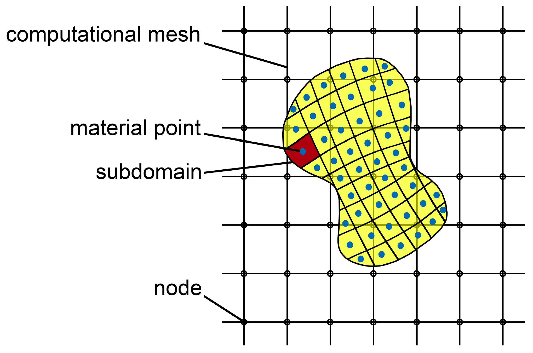
The material point method was originally proposed by Sulsky et al. [44] to model problems of solid mechanics involving large deformations. In this approach, the continuum medium is discretized as a set of subdomains, named material points (Figure 1). The material point is a Lagrangian point, in which any information pertaining the subdomain is concentrated, such as density, acceleration, velocity, displacement, mechanical characteristics, external loads and state variables.
Each material point moves attached to the solid skeleton. This aspect provides the Lagrangian description of the continuum. To solve the governing equations, the material points are overlaid on a computational mesh (Eulerian mesh) which is usually kept undeformed during the whole simulation and does not carry any information. This mesh has to be built to cover the entire space where the material points are expected to move during simulation.
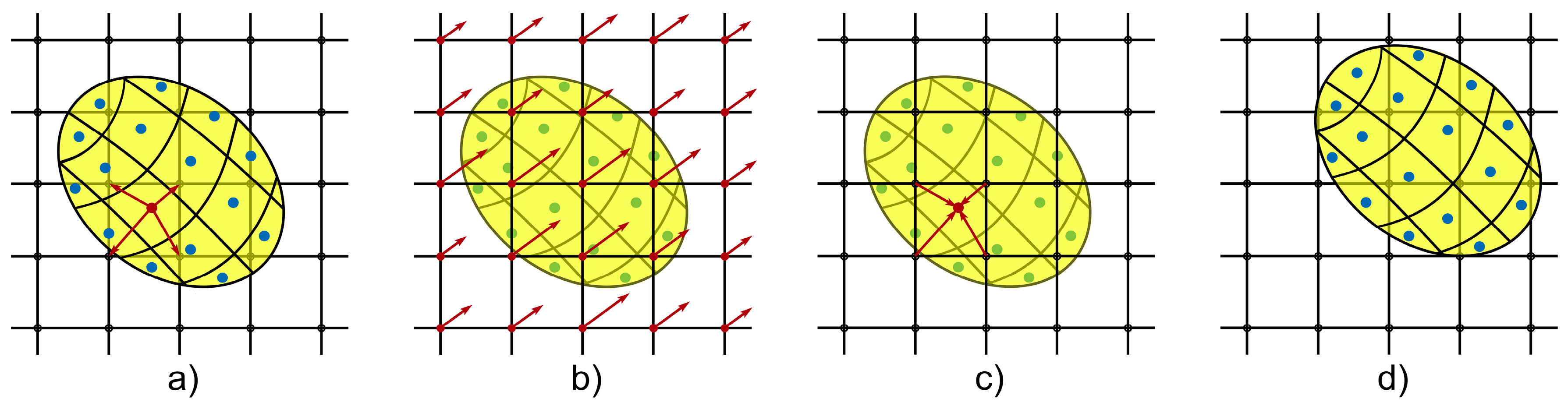
The calculation scheme of MPM for a single time step is shown in Figure 2. At the beginning of each time step, information is transferred from the material points to the mesh nodes using interpolation shape functions (Figure 2a). Then, the governing equations are solved at the nodes to obtain the nodal accelerations (Figure 2b), and the resulting values are used in order to update accelerations, velocities and displacements of the material points and to calculate stresses and deformations of them (Figure 2c). Finally, the position of the material points is updated before considering the next time step (Figure 2d). No information associated with the mesh is required. In this way, large displacements are calculated with the mesh remaining undeformed during the numerical simulation. This ensures the solution accuracy even when the material points undergo large displacements. In conclusion, MPM allows overcoming the limitations of the Eulerian and Lagrangian approaches. If compared with the Eulerian approach, the computational cost is substantially reduced. In addition, the mesh distortion problems are avoided unlike in the Lagrangian approach.
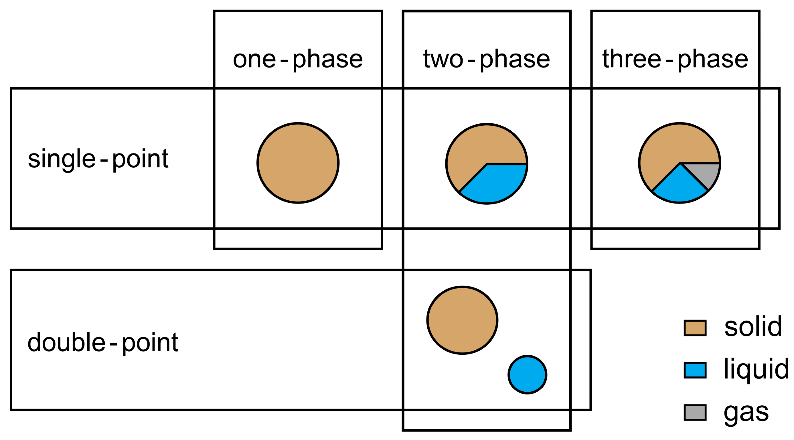
Two different formulations of MPM can be distinguished: the single-point formulation and the double-point one (Figure 3). In the single-point formulation, soil is considered as a unique medium that is discretized by a set of material points. Each material point represents both solid and fluid phases. Dry soils, pure liquids and saturated soils under fully drained or undrained conditions can be modelled using the one-phase single-point formulation [34,35,45,46]. On the contrary, the behaviour of saturated soils and unsaturated soils under transient conditions should be modelled using the two-phase single-point formulation [36,47] and the three-phase single-point formulation [48,49], respectively. In these approaches, a set of material points is again used, with the fluid pressures that are considered as additional variables.
In the double-point formulation, solid and fluid phases are represented separately by means of two distinct sets of material points. Each material point carries only information of the phase that it represents. This approach is suitable to analyse engineering problems where the pore fluids move separately from the solid phase [32,50]. However, this latter formulation is much more expensive from a computational viewpoint than the single-point formulation.
In the present study, the single-point formulation is used. Specifically, the one-phase single-point formulation is employed to model the soil behaviour above the groundwater level, and the two-phase single-point formulation is used when the soil is submerged in water, and the effects of the relative motion between solid and water phases are considered not significant [29,47]. Both formulations are implemented in the Anura3D software (developed by the Anura3D MPM Research Community [51]), which was used herein to perform the analysis presented in the subsequent section.
3. Run-Out Simulation of the Cook Lake Landslide
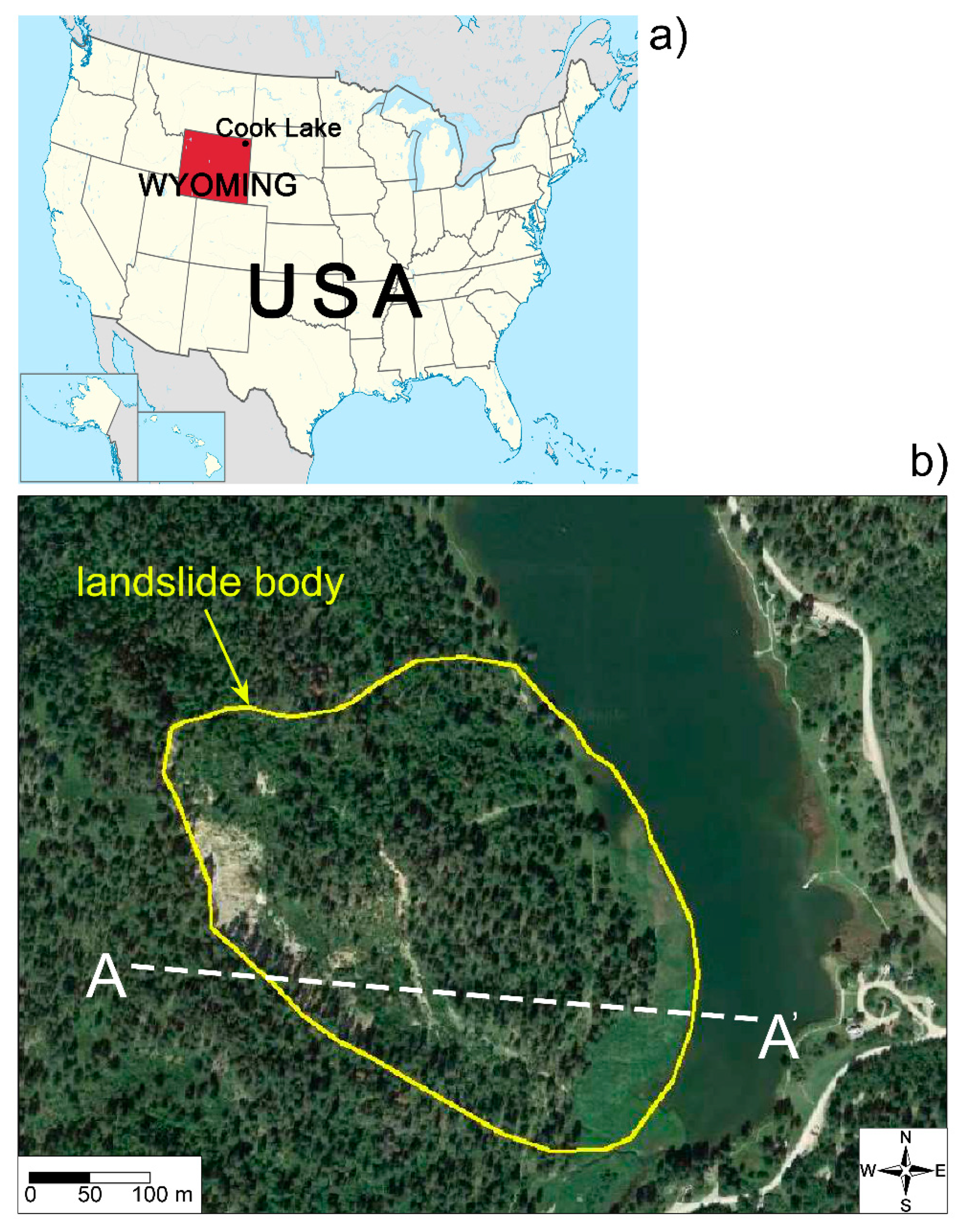
In this section, a landslide that occurred in 1997 at Cook Lake, WY, USA, is considered (Figure 4). This landslide was triggered by a significant increase in the groundwater level after a long rainy period involving the two preceding years. Several studies are available in the literature, in which a detailed description of the landslide is provided along with an analysis of the failure process that occurred in the slope [41,42,43]. According to the classification by Cruden and Varnes [52], this landslide can be categorised essentially as a translation slide. The size of the landslide was about 420 m in width and 380 m in length (Figure 4), with a height of the head scarp of about 15 m. The outline of the landslide is documented by Scheevel et al. [42] and highlighted in Figure 4, for the sake of completeness. The subsoil of the Cook Lake area consists of three different geological formations: Lakota Formation, Morrison Formation and Redwater Member [53]. Lakota Formation, of Cretaceous origin, is made up of claystone, siltstone and conglomeratic sandstone. Morrison Formation consists mainly of siltstone and claystone. Finally, Redwater Member is made up of shale, glauconite, sandstone and limestone. Both Morrison Formation and Redwater Member are of Jurassic age. The landslide involved mainly the Morrison Formation and Redwater Member, whereas the Lakota Formation was slightly involved. Both Morrison Formation and Redwater Member exhibited a soil-like behaviour due to a weathering process that affected these units [41]. In particular, on the basis of the Atterberg limits, the Morrison Formation can be classified as a low-plasticity silt, and the Redwater Member as a low-plasticity clay [41].
Unit weight γ, intercept cohesion c’ and angle of shearing resistance φ’ of the Morrison Formation and Redwater Member are shown in Table 1. These strength parameters were obtained from laboratory tests documented in the published studies [41,42,43]. Many soil samples were taken at different depths from the ground surface to the slip surface. Afterwards, these samples were subjected to direct shear tests. Specifically, 12 samples were taken from the Morrison Formation and 16 from the Redwater Member [41]. Every soil sample was subjected to different cycles of sharing to determine the residual shear strength parameters [41]. The soil properties used in the present study were directly provided by Santi et al. [41]. They can be seen as representative parameters of the above-mentioned formations. On the contrary, geotechnical data concerning the Lakota Formation are not available.
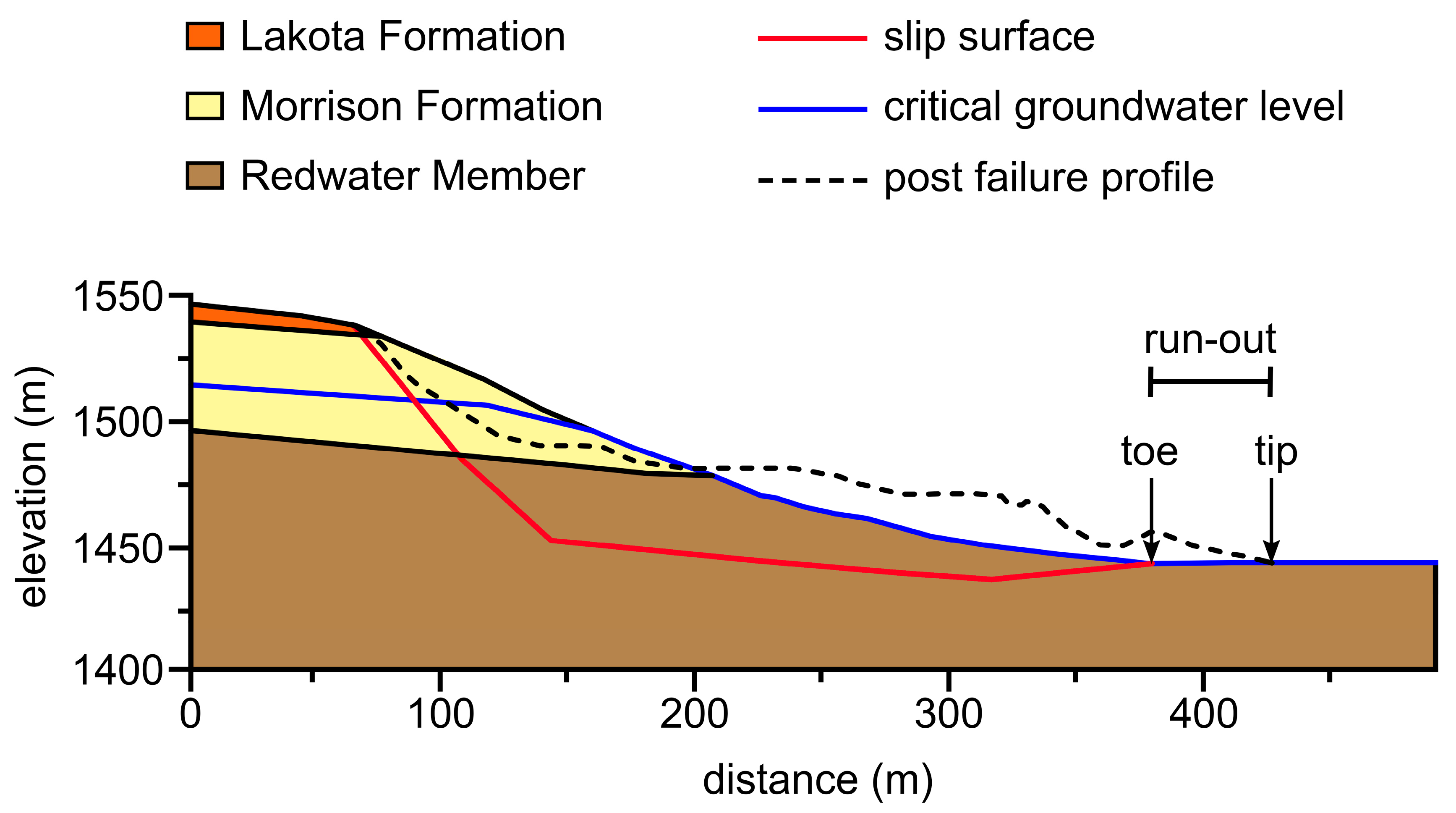
A schematic geological section of the slope is presented in Figure 5. It refers to the cross-section A-A’ the trace of which is indicated in Figure 4. The topographic profile shown in Figure 5 refers to the pre-failure condition, and was acquired from the USGS National Elevation Database [41]. As can be seen from this figure, the Lakota Formation practically was not involved in the landslide body. The subsoil model also shows the slip surface location reconstructed by the authors of [41,42], along with the topographic profile of the slope detected after the event and the run-out distance of the landslide (defined as the distance between the toe of the slip surface and the tip of the displaced material). The slip surface was located at an average depth of about 30 m, with a maximum depth of 50 m in the upper zone of the slope (Figure 5). The post-failure profile was reconstructed on the basis of the 1-ft resolution survey produced by the U.S Forest Service [41].
According to Santi et al. [41] and Scheevel et al. [42], after a rainy period of two years, a large portion of the subsoil was submerged in water due to an increase in the groundwater level. The critical groundwater level corresponding to the slope failure was established by the above-mentioned authors on the basis of field observations and the results of a back-analysis carried out using the limit equilibrium approach. The location of this critical level is also indicated in Figure 5. For a more complete understanding of the deformation processes of the Cook Lake landslide, the post-failure stage is analysed in this study using the material point method implemented in the Anura3D software [51].
The analysis was carried out under plane-strain conditions, referring to the section A-A’ indicated in Figure 4. The starting point of this analysis is the slope condition represented in Figure 5. In addition, Figure 6 shows the adopted computational mesh with an indication of the unstable soil mass delimited by the slip surface, and the location of the critical groundwater level, as documented in the paper by Scheevel et al. [42].
The mesh is made up of triangular elements with an average size of 3 m. This value was selected as the maximum element size capable to provide converging results, in accordance with the results of a sensitivity analysis preventively carried out in the present study. The initial distribution of the material points was three points per element. Boundary conditions were simulated by rollers on the left and right vertical sides of the model to constrain the horizontal displacements, and by hinges located at the bottom where both vertical and horizontal displacements were prevented. The one-phase single-point formulation was used for the soils above the groundwater level, which are hence considered as dry materials with nil pore water pressure. In other words, the effects of the partial saturation of this slope portion are disregarded. The two-phase single-point formulation was used for the submerged soils. Therefore, it is assumed that water moves attached to the solid skeleton, and pore water pressure is an additional variable. A hydrostatic water pressure distribution is assumed in the calculations. Since an explicit dynamic formulation was employed in ANURA3D to solve the governing equations, the solution was conditionally stable. Therefore, a time-step less than a critical value must be used in the calculations to ensure numerical stability. This critical value can be assessed according to the Courant–Friedrichs–Levy condition [54]. However, when the two-phase single-point formulation is used, the critical time-step Δt is strongly influenced by the hydraulic conductivity, k. Specifically, the lower k, the lower Δt and consequently the higher the computational costs. Therefore, a high value of k is assumed (k = 0.01 m/s) in the present study to reduce the calculation time [55]. As a consequence, the analysis was carried out under drained conditions, and excess pore water pressures that may have occurred during sliding were ignored. It was found that a value of Δt = 0.01 s is sufficient to satisfy the stability condition for the case study under consideration.
The initial stress state of the slope was generated using the well-known gravity loading procedure under the hypothesis that the involved soils behave as linear elastic materials. Since Young’s modulus E’ and Poisson’s ratio ν’ were not available, typical values of these parameters were used in the calculations. Specifically, Young’s modulus is assumed to be equal to 60 MPa and 70 MPa for the Morrison Formation and Redwater Member, respectively [56], with ν’ = 0.3 for all involved materials. The authors also ascertained that a different choice of E’ and ν’ (satisfying the afore-mentioned stability condition) did not significantly affect the conclusions of the present study. After generating the initial stress state, the post-failure stage of the landslide was simulated by employing an elastic perfectly plastic Mohr–Coulomb model in conjunction with a non-associated flow rule to model the behaviour of the materials involved in the landslide body. In this connection, the values of the shear strength parameters in Table 1 were used. Furthermore, the angle of dilation was assumed to be nil. On the contrary, a linearly elastic behaviour was kept for the soils outside the landslide body shown in Figure 6. In this way, the soil mass delimited by the slip surface became unstable due to the pore water pressures acting on the slip surface, and was left free to move downwards until a new condition of equilibrium was attained. Different analyses were performed to analyse the effects of the groundwater table location on the run-out process of the landslide. It was found that the best agreement between prediction and observation was obtained when the critical groundwater table shown in Figure 5 and Figure 6 was considered. The respective results are documented in Figure 7, Figure 8 and Figure 9.
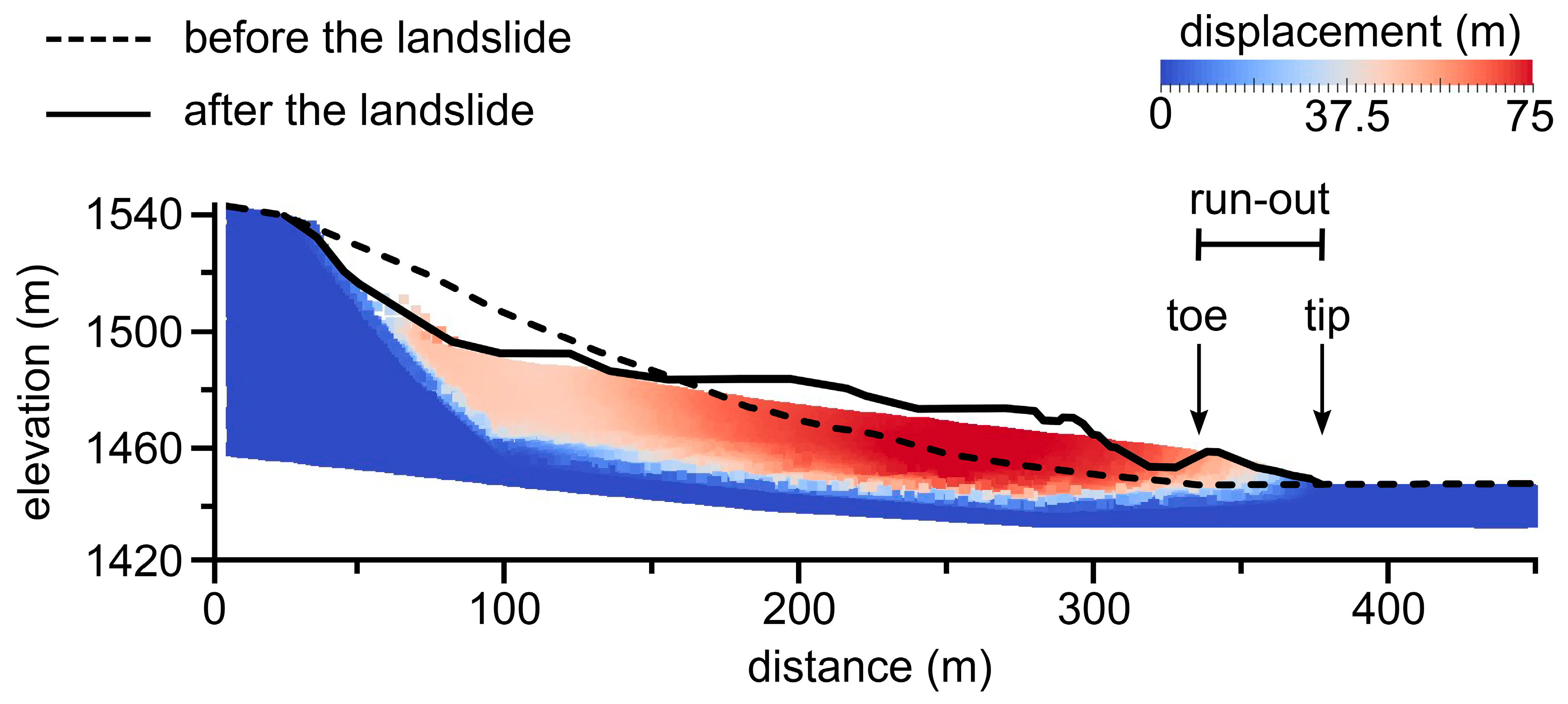
Specifically, Figure 7 shows the final configuration of the displaced material provided by the numerical simulation. The original ground surface and the slope profile detected just after the landslide are also shown in this figure, for the sake of comparison. As can be seen, the post-failure configuration obtained from the numerical simulation is in satisfactory agreement with the observed one. The maximum difference between the calculated and the measured profiles is on the order of a few meters. The run-out distance, the depletion zone and the deposition one obtained from the numerical simulation are very similar to those actually observed. In particular, a run-out distance of about 50 m is evaluated with the cumulated displacement attaining a maximum value of about 75 m (Figure 7). These results also prove that the simplified assumptions made in the present study are reasonable. Specifically, the effects of the partial saturation of the soils above the groundwater table and those of the excess pore water pressures built up during sliding (which have been ignored in the present analysis) should not have significantly affected the run-out process of the considered landslide. In other words, these effects seem to have played a role of minor importance in the present case study.
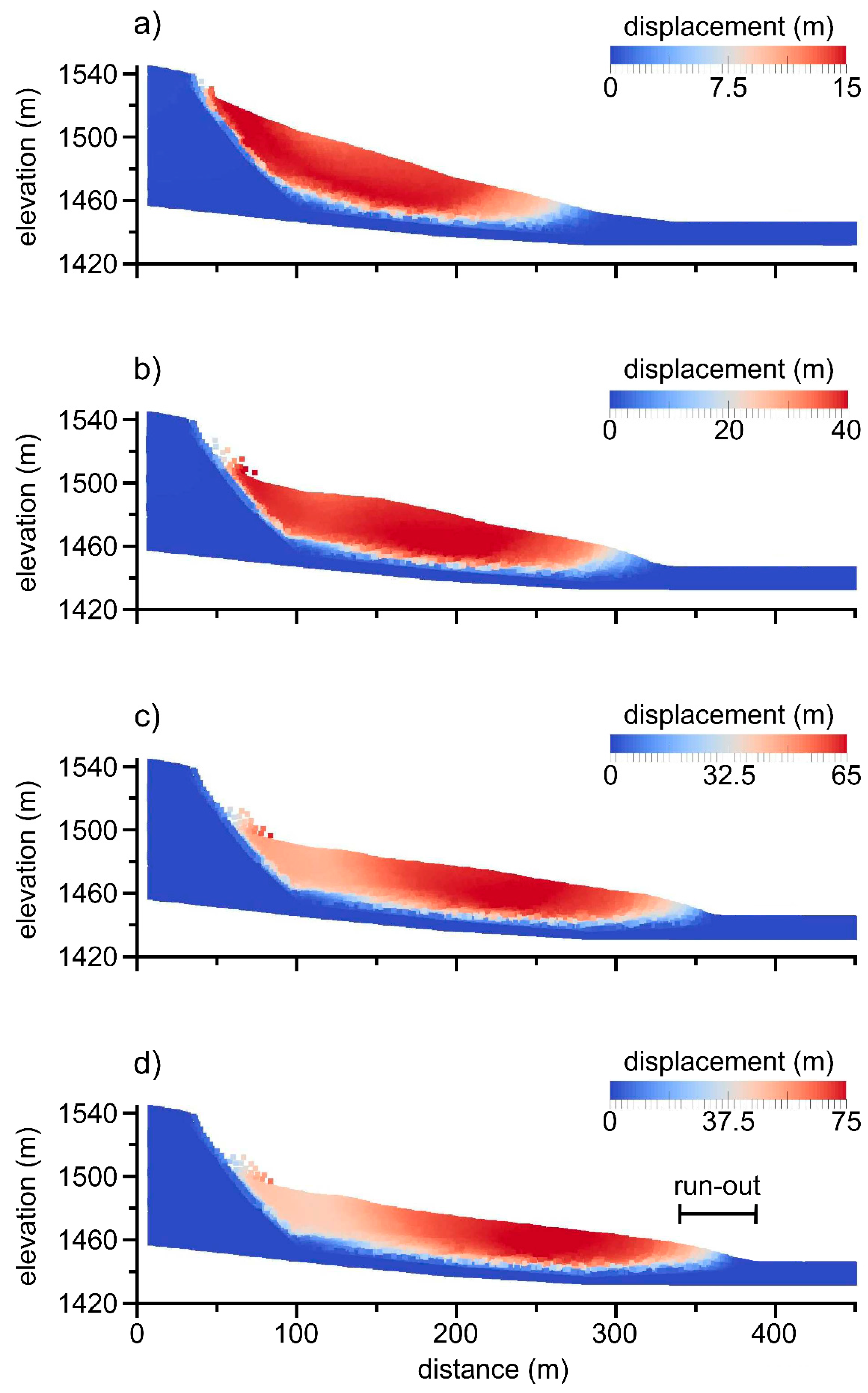
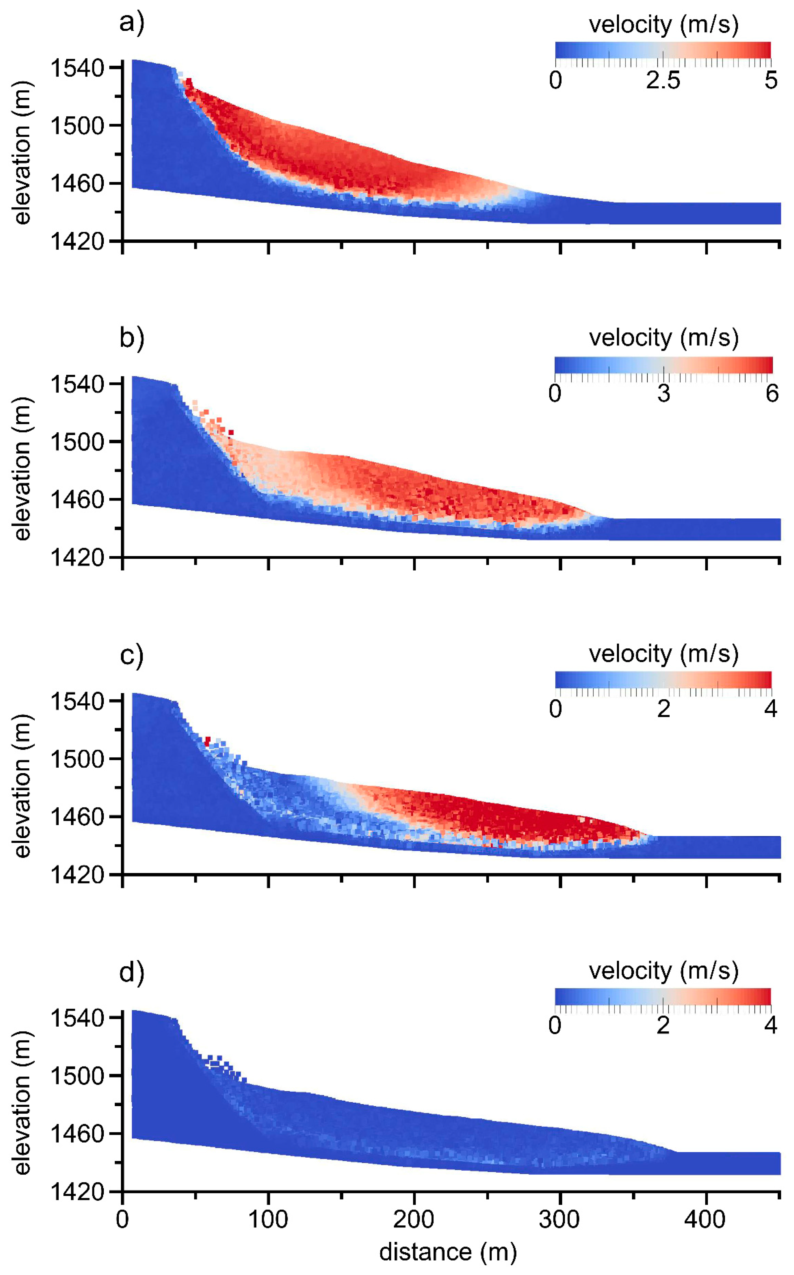
Finally, Figure 8 and Figure 9 show the evolution of the landslide at different times, in terms of displacement (Figure 8) and velocity (Figure 9) of the material points. Starting from a configuration just after the slope failure (Figure 8a), the landslide body moved essentially as a translational slide (Figure 8b,c) until the soil mass reached a condition of equilibrium (Figure 8d). The maximum thickness of the displaced material was approximately 35 m. The sliding mass velocity was initially in the order of 3–5 m/s (Figure 9a). With increasing time, velocity attained a maximum value of 6 m/s in the lower zone of the landslide body (Figure 9b), which was also the last portion of the sliding soil mass to stop (Figure 9c).
Summarizing, the obtained results confirm the exact location of the critical groundwater level found by Scheevel et al. [42] and highlight the important role played by the associated pore water pressures on the post-failure behaviour of the Cook Lake landslide.
4. Discussion
This paper deals with the modelling of problems involving large displacements in the geotechnical engineering field. Specifically, attention is focused on the post-failure stage of landslides whose analysis is often ignored in engineering practice. Indeed, deformation and failure mechanisms of slopes, which are generally classified in pre-failure, failure, post-failure and reactivation stages, are commonly analysed by means of simplified methods or traditional numerical techniques. Among simplified methods, the limit equilibrium method is the most widely employed for analysing the failure stage. As well known, it only allows the evaluation of a safety factor to express the overall stability conditions of the slope. Instead, traditional numerical techniques, such as the finite element method or the finite difference method, are usually employed for simulating the pre-failure stage as well as the failure and reactivation phases. However, these techniques are affected by severe drawbacks when the calculated deformations and displacements take high values, as usually happens in the post-failure stage of many landslides. In these circumstances, a mesh distortion can occur with a consequent loss of accuracy of the solution and underestimation of the soil displacements. Different numerical techniques have been developed in recent years to overcome these limitations. Among them, MPM is particularly suitable to analyse real problems involving large displacements.
In the present study, this method is used to analyse the post-failure stage of the Cook Lake landslide in order to complete the understanding of the deformation processes occurred during this landslide. The obtained results confirm the suitability and capability of MPM to provide useful information on the kinematics of the moving soil mass and on the entire run-out process of the displaced material. This represents a good perspective from an engineering point of view, since the above-mentioned information could be particularly useful for establishing the most adequate stabilization measures and minimizing the risk of catastrophic damages [57].
5. Conclusions
This paper focuses attention on a landslide that occurred at Cook Lake (WY, USA), which was triggered by an increase in the groundwater level owing to rainfall. Several studies were published on this landslide, where useful data can be found such as the location of the groundwater level at the time of the slope collapse. To provide a more complete understanding of the deformation processes occurred, the post-failure stage is analysed in the present study using MPM, which is an advanced numerical technique capable of dealing with large deformation problems. The final configuration of the displaced material provided by the numerical simulation effectively matches the profile detected after the landslide, when the above-mentioned critical groundwater level is accounted for. In addition, some kinematical aspects of the run-out process are highlighted to provide further information about the considered landslide. This study also shows that an adequate analysis of the post-failure stage and a reliable prediction of the landslide kinematics are very useful for better understanding the deformation mechanisms of the landslides and consequently minimizing the associated risk.
Author Contributions
Conceptualization, A.T., E.C. and L.P.; MPM analysis, L.P.; writing—original draft preparation, A.T. and L.P.; writing—review and editing, A.T. and E.C.; supervision, A.T. and E.C. All authors contributed equally to the preparation of this work. All authors have read and agreed to the published version of the manuscript.
Funding
This research received no external funding.
Conflicts of Interest
The authors declare no conflict of interest.
References
- Hungr, O.; Leroueil, S.; Picarelli, L. The Varnes classification of landslide types, an update. Landslides 2014, 11, 167–194. [Google Scholar] [CrossRef]
- Iverson, R.M.; George, D.L.; Allstadt, K.; Reid, M.E.; Collins, B.D.; Vallance, J.W.; Schilling, S.P.; Godt, J.W.; Cannon, C.M.; Magirl, C.S.; et al. Landslide mobility and hazards: Implications of the 2014 Oso disaster. Earth Planet. Sci. Lett. 2015, 412, 197–208. [Google Scholar] [CrossRef] [Green Version]
- Corominas, J.; Moya, J.; Ledesma, A.; Lloret, A.; Gili, J.A. Prediction of ground displacements and velocities from groundwater level changes at the Vallcebre landslide (Eastern Pyrenees, Spain). Landslides 2005, 2, 83–96. [Google Scholar] [CrossRef]
- Conte, E.; Donato, A.; Pugliese, L.; Troncone, A. Kinematics of the Maierato Landslide (Calabria, Southern Italy). Procedia Eng. 2016, 158, 194–199. [Google Scholar] [CrossRef] [Green Version]
- Leroueil, S. Natural slopes and cuts: Movement and failure mechanisms. Géotechnique 2001, 51, 197–243. [Google Scholar] [CrossRef]
- Duncan, J.M. State of the art: Limit equilibrium and finite-element analysis of slopes. J. Geotech. Eng. 1996, 122, 577–596. [Google Scholar] [CrossRef]
- Gottardi, G.; Butterfield, R. Modelling 10 years of downhill creep data. In Proceedings of the 15th International Conference on Soil Mechanics and Geotechnical Engineering, Istanbul, Turkey, 27–31 August 2001; Volume 1–3, pp. 27–31. [Google Scholar]
- Conte, E.; Donato, A.; Troncone, A. A simplified method for predicting rainfall-induced mobility of active landslides. Landslides 2017, 14, 35–45. [Google Scholar] [CrossRef]
- Conte, E.; Troncone, A. A performance-based method for the design of drainage trenches used to stabilize slopes. Eng. Geol. 2018, 239, 158–166. [Google Scholar] [CrossRef]
- Conte, E.; Troncone, A. Analytical method for predicting the mobility of slow-moving landslides owing to groundwater fluctuations. J. Geotech. Geoenviron. Eng. ASCE 2011, 137, 777–784. [Google Scholar] [CrossRef]
- Conte, E.; Troncone, A. A method for the analysis of soil slips triggered by rainfall. Géotechnique 2012, 62, 187–192. [Google Scholar] [CrossRef]
- Conte, E.; Troncone, A. Stability analysis of infinite clayey slopes subjected to pore pressure changes. Géotechnique 2012, 62, 87–91. [Google Scholar] [CrossRef]
- Potts, D.M.; Dounias, G.T.; Vaughan, P.R. Finite element analysis of progressive failure of Carsington embankment. Géotechnique 1990, 40, 79–101. [Google Scholar] [CrossRef]
- Griffiths, D.L.; Lane, P.A. Slope stability analysis by finite element. Géotechnique 1999, 49, 387–403. [Google Scholar] [CrossRef]
- Troncone, A. Numerical analysis of a landslide in soils with strain-softening behaviour. Géotechnique 2005, 55, 585–596. [Google Scholar] [CrossRef]
- Troncone, A.; Conte, E.; Donato, A. Two and three-dimensional numerical analysis of the progressive failure that occurred in an excavation-induced landslide. Eng. Geol. 2014, 183, 265–275. [Google Scholar] [CrossRef]
- Conte, E.; Donato, A.; Pugliese, L.; Troncone, A. Analysis of the Maierato landslide (Calabria, Southern Italy). Landslides 2018, 15, 1935–1950. [Google Scholar] [CrossRef]
- Crosta, G.B.; Imposimato, S.; Roddeman, D.G. Numerical modelling of large landslide stability and runout. Nat. Hazards Earth Syst. Sci. 2003, 3, 523–538. [Google Scholar] [CrossRef]
- Tang, H.M.; Liu, X.; Hu, X.L.; Griffiths, D.V. Evaluation of landslide mechanisms characterized by high-speed mass ejection and long-run-out based on events following the Wenchuan earthquake. Eng. Geol. 2015, 194, 12–24. [Google Scholar] [CrossRef]
- Zhang, X.; Krabbenhoft, K.; Sheng, D.; Li, W. Numerical simulation of a flow-like landslide using the particle finite element method. Comput. Mech. 2015, 55, 167–177. [Google Scholar] [CrossRef]
- Calvetti, F.; di Prisco, C.; Vairaktaris, E. DEM assessment of impact forces of dry granular masses on rigid barriers. Acta Geotech. 2017, 12, 129–144. [Google Scholar] [CrossRef]
- Scaringi, G.; Fan, X.; Xu, Q.; Liu, C.; Ouyang, C.; Domènech, G.; Yang, F.; Dai, L. Some considerations on the use of numerical methods to simulate past landslides and possible new failures: The case of the recent Xinmo landslide (Sichuan, China). Landslides 2018, 15, 1359–1375. [Google Scholar] [CrossRef]
- Bui, H.H.; Fukagawa, R.; Sako, K.; Wells, J.C. Slope stability analysis and discontinuous slope failure simulation by elasto-plastic smoothed particle hydrodynamics (SPH) (DPmodel). Géotechnique 2011, 61, 565–574. [Google Scholar] [CrossRef]
- Pirulli, M.; Pastor, M. Numerical study on the entrainment of bed material into rapid landslides. Géotechnique 2012, 62, 959–972. [Google Scholar] [CrossRef]
- Pastor, M.; Haddad, B.; Sorbino, G.; Cuomo, S.; Drempetic, V. A depth-integrated, coupled SPH model for flow-like landslides and related phenomena. Int. J. Numer. Anal. Methods Geomech. 2009, 33, 143–172. [Google Scholar] [CrossRef]
- Dai, Z.; Huang, Y.; Cheng, H.; Xu, Q. 3D numerical modeling using smoothed particle hydrodynamics of flow-like landslide propagation triggered by the 2008 Wenchuan earthquake. Eng. Geol. 2014, 180, 21–33. [Google Scholar] [CrossRef]
- Zabala, F.; Alonso, E.E. Progressive failure of Aznalcollar dam using the material point method. Géotechnique 2011, 61, 795–808. [Google Scholar] [CrossRef]
- Solowski, W.T.; Sloan, S.W. Evaluation of material point method for use in geotechnics. Int. J. Numer. Anal. Methods Geomech. 2015, 39, 685–701. [Google Scholar] [CrossRef]
- Alonso, E.E.; Yerro, A.; Pinyol, N.M. Recent developments of the material point method for the simualtion of landslides. IOP Conference Series 26, 012003. In Proceedings of the International Symposium on Geohazards and Geomechanics, Warwick, UK, 10–11 September 2015. [Google Scholar]
- Bhandari, T.; Hamad, F.; Moormann, C.; Sharma, K.G.; Westrich, B. Numerical modelling of seismic slope failure using MPM. Comput. Geotech. 2016, 75, 126–134. [Google Scholar] [CrossRef]
- Li, X.; Wu, Y.; He, S.; Su, L. Application of the material point method to simulate the post-failure runout processes of the Wangjiayan landslide. Eng. Geol. 2016, 212, 1–9. [Google Scholar] [CrossRef]
- Rohe, A.; Martinelli, M. Material point method and applications in geotechnical engineering. In Proceedings of the Conference Workshop on Numerical Methods in Geotechnics, Hamburg, Germany, 27–28 September 2017; pp. 57–72. [Google Scholar]
- Wang, B.; Vardon, P.J.; Hicks, M.A. Rainfall-induced slope collapse with coupled material point method. Eng. Geol. 2018, 239, 1–12. [Google Scholar] [CrossRef] [Green Version]
- Fern, J.; Rohe, A.; Soga, K.; Alonso, E. The Material Point Method for Geotechnical Engineering. A Practical Guide, 1st ed.; CRC Press: Boca Raton, FL, USA, 2019. [Google Scholar]
- Conte, E.; Pugliese, L.; Troncone, A. Post-failure stage simulation of a landslide using the material point method. Eng. Geol. 2019, 253, 149–159. [Google Scholar] [CrossRef]
- Troncone, A.; Conte, E.; Pugliese, L. Analysis of the Slope Response to an Increase in Pore Water Pressure Using the Material Point Method. Water 2019, 11, 1446. [Google Scholar] [CrossRef] [Green Version]
- Yerro, A.; Soga, K.; Bray, J. Runout evaluation of Oso landslide with the material point method. Can. Geotech. J. 2019, 56, 1304–1317. [Google Scholar] [CrossRef] [Green Version]
- Conte, E.; Pugliese, L.; Troncone, A. Post-failure analysis of the Maierato landslide using the material point method. Eng. Geol. 2020, 277, 105788. [Google Scholar] [CrossRef]
- Soga, K.; Alonso, E.; Yerro, A.; Kumar, K.; Bandara, S. Trends in large-deformation analysis of landslide mass movements with particular emphasis on the material point method. Géotechnique 2016, 66, 248–273. [Google Scholar] [CrossRef] [Green Version]
- Zhang, X.; Chen, Z.; Liu, Y. The Material Point Method: A Continuum-Based Particle Method for Extreme Loading Cases; Elsevier: London, UK, 2017. [Google Scholar]
- Santi, P.; Scheevel, C.; Bradford, E. Summary Report–Stability Analysis of Cook Lake Landslide Crook County, Wyoming; Colorado School of Mines, Department of Geology and Geological Engineering: Golden, CO, USA, 2016. [Google Scholar]
- Scheevel, C.; Santi, P.; Emmanuel, K. Stability and Runout Analysis of the Cook Lake Landslide, Wyoming. In Proceedings of the 3rd North American Symposium on Landslides, Roanoke, VA, USA, 4–8 June 2017; pp. 645–655. [Google Scholar]
- Santi, P. Landslide Analysis with Incomplete Data: Examples from Colorado and Wyoming. In Proceedings of the Rocky Mountain Geo-Conference, Golden, Colorado, 2 November 2018; ASCE: Golden, CO, USA, 2018; pp. 15–25. [Google Scholar]
- Sulsky, D.; Chen, Z.; Schreyer, H. A particle method for history-dependent materials. Comput. Methods Appl. Mech. Eng. 1994, 118, 179–196. [Google Scholar] [CrossRef]
- Fern, J.E.; de Lange, D.A.; Zwanenburg, C.; Teunissen, J.A.M.; Rohe, A.; Soga, K. Experimental and numerical investigations of dyke failures involving soft materials. Eng. Geol. 2017, 219, 130–139. [Google Scholar] [CrossRef] [Green Version]
- Tran, Q.A.; Solowski, W. Generalized Interpolation Material Point Method modelling of large deformation problems including strain-rate effects–Application to penetration and progressive failure problems. Comput. Geotech. 2019, 106, 249–265. [Google Scholar] [CrossRef]
- Yerro, A.; Alonso, E.; Pinyol, N. Run-out of landslides in brittle soils. Comput. Geotech. 2016, 80, 427–439. [Google Scholar] [CrossRef] [Green Version]
- Yerro, A.; Alonso, E.; Pinyol, N. The material point method for unsaturated soils. Géotechnique 2015, 65, 201–217. [Google Scholar] [CrossRef] [Green Version]
- Bandara, S.; Ferrari, A.; Laloui, L. Modelling landslides in unsaturated slopes subjected to rainfall infiltration using material point method. Int. J. Numer. Anal. Meth. Geomech. 2016, 40, 1358–1380. [Google Scholar] [CrossRef]
- Bandara, S.; Soga, K. Coupling of soil deformation and pore fluid flow using material point method. Comput. Geotech. 2015, 63, 199–214. [Google Scholar] [CrossRef]
- Anura3D MPM Research Community. Available online: www.anura3d.com (accessed on 1 August 2020).
- Cruden, D.M.; Varnes, D.J. Landslides–Investigation and Mitigation; Special Report No. 247, Transportation Research Board; National Academy Press: Washington, DC, USA, 1996. [Google Scholar]
- Sutherland, W.M. Geologic Map of the Devil’s Tower 30′ × 60′ Quadrangle, Crook County, Wyoming, Butte and Lawrence Counties, South Dakota, and Carter County, Montana [Map]. 1:100,000; Wyoming State Geological Survey: Laramie, WY, USA, 2008. [Google Scholar]
- Courant, R.; Friedrichs, K.; Lewy, H. On the Partial Difference Equations of Mathematical Physics. IBM J. Res. Dev. 1967, 11, 215–234. [Google Scholar] [CrossRef]
- Yerro, A. MPM Modeling of Landslides in Brittle and Unsaturated Soils. Ph.D. Thesis, UPC, Barcelona, Spain, 2015. [Google Scholar]
- Obrzud, R.; Trury, A. The Hardening Soil Model—A Practical Guidebook; Z Soil.PC 100701 Report; Zace Services Ltd.: Lausanne, Switzerland, 2012. [Google Scholar]
- Cevasco, A.; Termini, F.; Valentino, R.; Meisina, C.; Bonì, R.; Bordoni, M.; Chella, G.P.; De Vita, P. Residual mechanisms and kinematics of the relict Lemeglio coastal landslide (Liguria, northwestern Italy). Geomorphology 2018, 320, 64–81. [Google Scholar] [CrossRef]
Figure 1.
Continuum medium discretization used in MPM with an indication of the computational mesh, the nodes and the material points.
Figure 1.
Continuum medium discretization used in MPM with an indication of the computational mesh, the nodes and the material points.

Figure 2.
MPM calculation scheme: (a) map information from material points to grid nodes; (b) solution of the governing equations at the nodes; (c) update of the material point information; (d) update of the material point position.
Figure 2.
MPM calculation scheme: (a) map information from material points to grid nodes; (b) solution of the governing equations at the nodes; (c) update of the material point information; (d) update of the material point position.

Figure 3.
Schematization of different approaches of MPM for a medium with different phases.

Figure 4.
The Cook Lake landslide: (a) location of Cook Lake; (b) aerial view of the landslide (after [42]).
Figure 4.
The Cook Lake landslide: (a) location of Cook Lake; (b) aerial view of the landslide (after [42]).

Figure 5.
Schematic geological section of the slope affected by the landslide (section A-A’, whose trace is indicated in Figure 4) with an indication of the slip surface, the topographic profile detected after the landslide and the critical groundwater level (after [42]). The toe of the slip surface, the tip of the displaced material and the run-out distance are also indicated.

Figure 6.
Computational mesh of the slope with an indication of the unstable soil mass bounded by the slip surface, and the location of the critical groundwater level that caused slope failure.
Figure 6.
Computational mesh of the slope with an indication of the unstable soil mass bounded by the slip surface, and the location of the critical groundwater level that caused slope failure.

Figure 7.
Final configuration of the slope obtained from the MPM simulation, with an indication of the topographic profile observed before and after the landslide.
Figure 7.
Final configuration of the slope obtained from the MPM simulation, with an indication of the topographic profile observed before and after the landslide.

Figure 8.
Displacement of the material points at different times during the post-failure stage: (a) t = 5 s; (b) t = 10 s; (c) t = 15 s; (d) t = 25 s (final configuration).
Figure 8.
Displacement of the material points at different times during the post-failure stage: (a) t = 5 s; (b) t = 10 s; (c) t = 15 s; (d) t = 25 s (final configuration).

Figure 9.
Velocity of the material points at different times during the post-failure stage: (a) t = 5 s; (b) t = 10 s; (c) t = 15 s; (d) t = 25 s (final configuration).
Figure 9.
Velocity of the material points at different times during the post-failure stage: (a) t = 5 s; (b) t = 10 s; (c) t = 15 s; (d) t = 25 s (final configuration).


Table 1.
Material properties [42].
Table 1.
Material properties [42].
| Geological Unit | γ (kN/m3) | c’ (kPa) | φ’ (°) |
|---|---|---|---|
| Morrison Formation | 19 | 18 | 33 |
| Redwater Member | 20 | 28 | 14 |
© 2020 by the authors. Licensee MDPI, Basel, Switzerland. This article is an open access article distributed under the terms and conditions of the Creative Commons Attribution (CC BY) license (http://creativecommons.org/licenses/by/4.0/).
Share and Cite
MDPI and ACS Style
Troncone, A.; Pugliese, L.; Conte, E. Run-Out Simulation of a Landslide Triggered by an Increase in the Groundwater Level Using the Material Point Method. Water 2020, 12, 2817. https://doi.org/10.3390/w12102817
AMA Style
Troncone A, Pugliese L, Conte E. Run-Out Simulation of a Landslide Triggered by an Increase in the Groundwater Level Using the Material Point Method. Water. 2020; 12(10):2817. https://doi.org/10.3390/w12102817
Chicago/Turabian StyleTroncone, Antonello, Luigi Pugliese, and Enrico Conte. 2020. "Run-Out Simulation of a Landslide Triggered by an Increase in the Groundwater Level Using the Material Point Method" Water 12, no. 10: 2817. https://doi.org/10.3390/w12102817
Note that from the first issue of 2016, this journal uses article numbers instead of page numbers. See further details here.