Ecosystem Services under Climate Change Impact Water Infrastructure in a Highly Forested Basin

Abstract

Climate change can have critical impacts on ecosystem services (ESs) and their inter-relationships, especially for water-related services. However, there has been little work done on characterizing the current and future changes in these services and their inter-relationships under a changing climate. Based on the revised universal soil loss equation (RUSLE), the soil conservation service curve number model (SCS-CN), and the improved stochastic weather-generator-based statistical downscaled global climate models (GCMs), we examined two important water-related services, namely, the soil conservation (SC) service and the flood mitigation (FM) service, and their inter-relationship under baseline and future climate scenarios (Representative Concentration Pathways (RCPs) 4.5 and 8.5). We took the Upper Hanjiang River Basin (UHRB), which is the core water source area of the China’s South-to-North Water Diversion Project (S–NWDP), as an illustration. The findings revealed that (1) the SC and FM services will both decrease under the two climate scenarios examined; (2) the SC and FM services showed a significant synergistic inter-relationship and the synergy will be improved by 16.48% and 2.95% under RCP 4.5 and RCP 8.5, respectively, which provides an opportunity for management optimization; (3) the ecological degradation in the UHRB will likely have serious consequences for the middle and lower reaches of the Hanjiang river basin, and therefore impact the actual economic benefits of the S–NWDP. This study points to the necessity for understanding the dynamic changes and inter-relationships of ecosystem services under future climate change and provides information regarding the consequences of climate change, which is useful for policy and infrastructure investment.

1. Introduction

Natural ecosystems are being affected by changing climate conditions through changes in ecosystem processes and ecosystem functioning [1,2]. The projected changes in climate pose a growing threat to ecosystems and biodiversity, which is predicted to become more severe in the coming decade [3]. Ecosystems become vulnerable and less resilient when the external stressors are beyond the level of the system’s self-regulation, affecting the distribution and amounts of ecosystem service (ES) benefits humans gain from nature [4]. The relationships between multiple ESs can be categorized as synergies (i.e., both an increase or a decrease) and trade-offs [5]. Synergies occur in situations in which two or more ESs increase or decrease at the same time, while trade-offs occur when an increase in the supply of one ES occurs at the cost of another. Both trade-offs and synergies may occur in response to the same driving factor [5] and they may change with changes in the ecosystem processes over time [6]. A better understanding of the spatial and temporal variations in ESs and their inter-relationships can inform stakeholders interested in optimizing synergies and reducing undesirable trade-offs, resulting in win–win strategies for ecologically sustainable development [7,8]. Failure to take account of changes in individual ESs and their interactions can result in sub-optimal planning for investments, particularly in a natural resource management infrastructure. In this study, we aimed to quantify the variations of ESs and the inter-relationships between them at spatial and temporal scales under different climate change scenarios.

Ecosystem shifts resulting from changes in external stressors are shaped by the resilience of the ecosystems, which may be altered by climate change [1]. Climate change impacts on ecosystems can occur as a slow dynamic process that is closely linked to a change in the regulating services [5]. A reduction in regulating services can weaken the ecosystem resilience [9]. Improving regulating ecosystem services can increase the production of provisioning and cultural services, for example, forest restoration can increase carbon storage, improve soil and water conservation, and provide an additional habitat [10]. There is increasing attention being paid to the projected change in provisioning services related to goods and services that are directly obtained from ecosystems; however, it is less clear how the underpinning regulating services may change with future climate projections.

Regulating services are abundant in the complex topographical environments with a high vegetation coverage and rich biodiversity in highly forested and high-altitude river basins. Forest ecosystems in watersheds are closely connected to the supply of hydrological regulation services throughout river basins [11]. Evaluating the variability of regulating services in river basins under climatic change is essential for policy formation toward ecological resilience at regional and global scales [12]. Changes in climate can interfere with ecosystem functions by altering eco-hydrologic processes [13] and subsequently triggering ecosystem regime shifts [14], altering the ecosystem service supply in watersheds [12]. Policy responses are likely to be needed to deal with water scarcity, water quality deterioration [15], floods, droughts, and water utilization clashes between local watersheds and water diversion projects. The starting points for changes leading to these problems are found in the soil- and water-related regulating services of the watershed. The soil management system is closely associated with water-regulating functions; however, increases in soil erosion caused by heavy rain, as well as landform features like topography at the watershed scale, can potentially modify evapotranspiration, infiltration, and some water regulation processes [16]. Moreover, soil erosion can reduce cropping productivity, cause water quality deterioration, and increase the probability of flooding and reservoir sedimentation, which interferes with the effective utilization of water at the site of interception [17,18]. The regulation of ESs in the upper reaches of watersheds may be critical to the optimization and economic viability of a downstream river infrastructure [19]. Understanding the changes in regulating services, such as soil conservation and flood mitigation in river basins, is essential for policy formation in relation to river and water management, including infrastructure planning.

Climate change can alter the quantity and spatio-temporal distribution of ESs [20] and their trade-offs [7,15], and a spatio-temporal assessment of the projected changes in an ES supply and trade-offs can contribute to ecosystem management and climate adaptation policy formulation [21,22]. Processes have been developed for evaluating the effects of climate change on the quantity and variability of ESs’ supply [23,24]. The study of the inter-relationships between ESs can assist stakeholders when exploring optimal ecosystem resource management scenarios [25]. However, little is known about how the inter-relationship between soil conservation (SC) and flood mitigation (FM) services will change as a result of climate-change-driven hydrological changes in watersheds, especially in climate-sensitive high-altitude basins [26]. Exploring the potential impact of the changing climate on ESs can also inform climate-related strategies that are used to mitigate the negative effects of climate change on human welfare [12]. Hence, it is essential to identify the spatio-temporal variations of ESs and changes in the pattern of inter-relationships between ESs under future climate scenarios [27].

Additionally, changes in ESs and their inter-relationships potentially impact built infrastructure such that key regulating ES changes under climate change scenarios should be considered as part of infrastructure investment planning. The South-to-North Water Diversion Project (S–NWDP) is the world’s largest water transfer project, transferring an average of 9.5 billion m³ yr⁻¹ of water from the Hanjiang River to supply 53.1 million people in Northern China [28,29]. The upper Hanjiang River Basin (UHRB) is the core water source area of the middle route of the S–NWDP, and the ecological health of the basin directly affects the quality and quantity of the water being transferred [30]. While a large amount of effort has been devoted to studying the water and environmental conditions downstream of the S–NWDP offtake [31,32], little is known about the ecological health of the water source area upstream from the S–NWDP offtake or of the implications for the scheme of ES changes in the upper basin. Estimations of the positive benefits of the scheme for sustainability may prove over-optimistic in the face of upstream climate change impacts [19].

We modeled future climate scenarios and the anticipated impacts on SC and FM services and their inter-relationship under a baseline climate scenario (2000–2015) and two different climate change scenarios (Representative Concentration Pathways (RCPs) 4.5 and 8.5) from 2030 to 2045. The objectives of this study were (1) to assess the spatio-temporal variation of ESs under different climate change scenarios, (2) to investigate the spatio-temporal heterogeneity in the inter-relationship of ESs under different climate change scenarios, and (3) to explore the ecological conditions in the UHRB and the implications for the S–NWDP due to climate change.

2. Data and Methods

2.1. Study Area

The Hanjiang River Basin is the largest tributary of the Yangtze River, and the Upper Hanjiang River (UHR) is the water source area of the Middle Route Project of the South-to-North Water Diversion in China [33,34]. The river extends over a length of 652 km through the west to east of the UHRB, covering 6.02 × 10⁴ km² and accounting for 39.76% of the Hanjiang River drainage area. The UHRB is a typical natural ecological zone [34] located in the center of China (Figure 1a) and is a high-value basin for socio-economic activity, biodiversity conservation, and ecological sustainability, both at the watershed and national scales. The northern end of the UHRB is bordered by the Qinling Mountain and the south is bordered by the Daba–Micang mountains. The study area consists of three sub-regions: the Qinling Mountain Region (QM), the Hanzhong–Ankang Hilly Region (H–AH), and the Daba Mountain Region (DM), with elevations varying from 157 to 3473 m (Figure 1b). The study area is characterized by undulating mountains and ravines, with a high vegetation coverage of natural woodland and grassland, which in total accounts for more than 74% of the land-cover type. The land-cover types in decreasing order of prevalence are as follows: grassland (41.00%) > forest (33.53%) > cropland (24.43%) > settlement (0.66%) > wetland (0.36%) > unused (0.02%) (Figure 1c). The study area is in the northern subtropical monsoon climate zone, where the annual mean precipitation is 653 to 1183 mm. The UHRB features beaded river basins and plains, and it has become an important industrial, agricultural, and commercial center in the hinterland of the Qinling–Daba region. In the UHRB, due to significant differences in the natural environment, including terrain, altitude, slope, and climatic conditions, the precipitation is mainly concentrated in summer and rainstorms occur frequently. Rainstorms can not only result in soil erosion, debris flow, and other eco-environmental problems [35] in the upstream reaches but also threaten water quality in the reservoir and the ecological security of the middle and lower Hanjiang River Basin [33], including immediately upstream of the offtake for the S–NWDP.

2.2. Soil Conservation Service Mapping

The amount of soil retention is commonly employed to assess the soil conservation service in ecosystems. Soil retention can be evaluated in terms of potential soil loss and actual soil loss [36] which are based on an empirical model, namely, the revised universal soil loss equation (RUSLE) [37,38], as follows:

$$SC=P_e-A_e,$$

(1)

$$P_e=R\times K\times L\times S,$$

(2)

$$A_e=R\times K\times L\times S\times C\times P,$$

(3)

where SC is the annual amount of soil conservation (t hm⁻² yr⁻¹), $P_e$ refers to the annual amount of potential soil erosion (t hm⁻² yr⁻¹), and $A_e$ is defined as the annual amount of actual soil erosion (t hm⁻² yr⁻¹). The other parameters were computed as follows:

$$R={{\displaystyle \sum }}_{i=1}^{12}1.735\times {10}^{(1.5\times \lg \left(\frac{P_i^2}{P}\right)-0.8188)},$$

(4)

$$K=\left\{0.2+0.3\times e^{\left[-0.0256\times S_a\left(1-\frac{S_i}{100}\right)\right]}\right\}{\left(\frac{S_i}{C_l+S_i}\right)}^{0.3}\left\{1.0-\frac{0.25C_o}{\left[C_o+e^{\left(3.72+2.95C_o\right)}\right]}\right\}\left\{1.0-\frac{0.7\times \left(1-\frac{S_a}{100}\right)}{\left(1-\frac{S_a}{100}\right)+e^{\left(-5.51+22.9\times \left(1-\frac{S_a}{100}\right)\right)}}\right\}\times 0.1317,$$

(5)

$$L={\left(\frac{\lambda }{22.13}\right)}^m m=\{\begin{array}{c}0.5 \theta \ge 5° \\ 0.4 5°>\theta \ge 3°\\ 0.3 3°>\theta \ge 1°\\ 0.2 1°>\theta \end{array},$$

(6)

$$S={\left(\frac{\sin \theta }{0.0896}\right)}^{0.6},$$

(7)

$$C=\{\begin{array}{c} 0 f>78.3\\ 0.6508-0.3436\times lg\left(f\right) 0<f\le 78.3\\ 1 f=0\end{array},$$

(8)

$$P=0.2+0.03\alpha ,$$

(9)

where R is the rainfall erosivity factor (MJ mm hm⁻² h⁻¹ yr⁻¹) that was evaluated using the Wischmeier and Smith empirical formula [38]; P_i and P are the monthly and annual precipitation (mm), respectively; K is the soil erodibility factor (t ha h h⁻¹ MJ⁻¹ mm⁻²) that was computed based on the Sharpley and Williams Erosion–Productivity Impact Calculator (EPIC) equation [39]; the proportion (%) of sand, silt, clay, and organic content in soil are expressed as $S_a$, $S_i$, $C_l$, and $C_o$, respectively; L is the slope length factor calculated by means of the equation proposed by McCool et al. [40]; $\theta$ is the angle of the slope in degrees; the crop and management factor $C$ is a dimensionless parameter obtained from the model developed by Cai et al. [41]; $f$ is the level of vegetation coverage; P is the soil retention factor [42]; $\alpha$ is the radiant slope steepness [43].

2.3. Flood Mitigation Service Mapping

The flood mitigation service was determined from the soil conservation service curve number (SCS-CN) model, which is widely used for evaluating the direct runoff depth [44] based on one single rainstorm event [45] under various scales and climatic situations [46]. Precipitation events greater than 50 mm within 24 h are regarded as rainstorms resulting in floods based on the storm standards of the Meteorological Department. The quantity of flood mitigation service is equal to the difference between the rainstorm and runoff:

$$\mathrm{FM}=R_s-Q$$

(10)

Based on water balance theory, the surface runoff can be computed as follows:

$$\{\begin{array}{c}Q=\frac{{\left(R_s-0.2S\right)}^2}{R_s+0.8S} R_s\ge 0.2S,\\ Q=0 R_s\le 0.2S,\end{array}$$

(11)

$$S=\frac{25400}{\mathrm{CN}}-254$$

(12)

where FM is the annual amount of flood mitigation service (mm); $R_s$ is the single-event precipitation (mm); $Q$ is the surface runoff (mm); S is the potential maximum rainwater amount retained by the soil before runoff; CN represents the capacity of the surface runoff, which is a dimensionless parameter related to the hydrologic soil group, LULC types, antecedent moisture conditions predicted from the rainfall of the previous five days, the permeability, and the topography [47]. The value of CN can be found from the National Engineering Handbook [48].

The annual single rainstorm days and storm days were obtained from the series data of daily precipitation events from 19 meteorological stations in the UHRB. The FM can be estimated using:

$$\mathrm{FM}=\left[R_s-\frac{{\left(R_s-0.2S\right)}^2}{R_s+0.8S}\right]\times R_d$$

(13)

where $R_d$ is the number of rainstorm days per year.

2.4. Change in Trends and the Inter-Relationship between ESs

The change in SC, FM, precipitation, and rainstorms in the UHRB from 2000 to 2015 and between 2030 and 2045 were quantified using a linear regression trend model. The linear regression trend model was used to explore the estimation trend of the variables over time based on a least-squares regression [49], which is a method that has been widely adopted to demonstrate that ecosystem and climate variation trends change as a continuous time series [50,51]. Integrating the linear trend (b) with the statistical significance level represented by p (0 < p < 1), the variables above were divided into five categories: significantly increased (b > 0 and p < 0.05), not significantly increased (b > 0 and p > 0.05), no change (b = 0), significantly decreased (b < 0 and p < 0.05), and not significantly decreased (b < 0 and p > 0.05).

The inter-relationship between two water-related ecosystem services in the three cases in the UHRB was detected using Pearson’s correlation coefficient analysis, which produces a test statistic based on covariance [52]. The statistic is denoted by r, the range of which is between −1 and 1. Overlaid with the significance level p, Pearson’s correlation analyses were processed with the function [r, p] = corr (X, Y) in MATLAB Version R2010b [50], where X and Y here represented the two water-related ecosystem services, namely, SC and FM, respectively. The inter-relationship between SC and FM was classified into five categories: significant synergy (r > 0 and p < 0.05), no significant synergy (r > 0 and p > 0.05), no inter-relationship (r = 0), significant trade-off (r < 0 and p < 0.05), and no significant trade-off (r < 0 and p > 0.05).

2.5. Future Climate Change Scenarios Generation

Future climate data of global climate models (GCMs) have been widely used to underpin investigations of the potential impact of climate change on surface processes and effective adaptation responses [22,53]. In this research, we used the statistical downscaling model, NWAI-WG (weather generator developed at New South Wales Department of Primary Industries, Wagga Wagga Agricultural Institute), developed by Liu and Zuo [54] based on the improved stochastic weather generator (WGEN) [55], to generate daily and specific site data. The future projected climate data were obtained from the Earth System Model of the GCM supplied by the Beijing Normal University (BNU-ESM) in the Coupled Model Intercomparison Project phase 5 (CMIP 5, https://pcmdi.llnl.gov/mips/cmip5/index.html) from the World Climate Research Program [56]. Two future greenhouse gas emission scenarios (GGESs) from 2030 to 2045 were used: RCP 4.5 (the intermediate emission scenario) [57] and RCP 8.5 (the high emission scenario) [58], which represent two ecological development models with a near-term stabilization of greenhouse gas emissions or rapid economic development with growing emissions, respectively. The integration of the GCMs and GGESs provides a representative range of potential climate conditions for the future [59]. The baseline period in our study was from 2000 to 2015.

The required daily precipitation data needed in this study was downscaled in three steps. First, the monthly climate change projection outputs from the BNU-ESM GCM with a spatial resolution of 2.8° × 2.8° were downscaled to the site scale (19 sites in the UHRB) through an inverse distance-weighted method. Second, the observed and raw GCM projected monthly data for the historical period, e.g., 1961–2000, for each site were then used to establish a relationship that was applied to correct the biases of the GCM-projected historical climate. Third, daily site-specific climate projections were generated from bias-corrected monthly outputs using a modified stochastic WGEN model [54]. The detailed description of our downscaling procedure can be found in [54].

2.6. Data and Materials

The data and materials adopted in this study are listed in

Table 1. The data and materials.

Datasets	Data Type	Spatial Resolution	Time Scale	Data Sources
Daily precipitation	Point	—	2000–2015	http://cdc.cma.gov.cn/
Soil properties	Raster	1 km	2000	http://westdc.westgis.ac.cn/data/
Soil texture	Raster	1 km	2008	China Soil-Map-Based Harmonized World
				Soil Database
DEM 1	Raster	30 m	2010	http://www.gdem.aster.ersdac.or.jp/
LULC 2	Polygon	30 m	2000, 2005, 2010	http://www.landcover.org/data/
	Raster	1 km	2015	http://www.gscloud.cn/
Runoff Curve Number	Value	—	1985	National Engineering Handbook
NDVI 3	Raster	250 m	2000–2015	http://ladsweb.nascom.nasa.gov/data/
GCM 4	Raster	2.8° × 2.8°	2030–2045	https://pcmdi.llnl.gov/mips/cmip5/index.html

¹ DEM refers to digital elevation model; ² LULC refers to land use and land cover; ³ NDVI refers to normalized difference vegetation index; ⁴ GCM refers to global climate model.

. The daily precipitation data for the baselines at 19 meteorological stations were obtained from the National Meteorological Information Center. Topographical parameters (i.e., the digital elevation model (DEM)) were derived from Shuttle Radar Topography Mission digital elevation data. The soil property and texture data were from the Chinese soil dataset based on the Harmonized World Soil Database version 1.1 [60]. The 250 m MODIS NDVI (moderate resolution imaging spectroradiometer, normalized difference vegetation index) data were acquired from NASA’s Earth Observing System. The LULC data were processed from the Landsat 5 Thematic Mapper data and the accuracy levels were above 94% according to site investigations and verification using Google Earth, which met the accuracy requirements of the ES simulation [61,62]. The value of CN was found in the National Engineering Handbook [48]. All the data were interpolated or resampled (all using a nearest neighbor assignment resampling algorithm, and a majority resampling algorithm for LULC data) to a 250 m spatial resolution before modeling [61,63].

3. Results

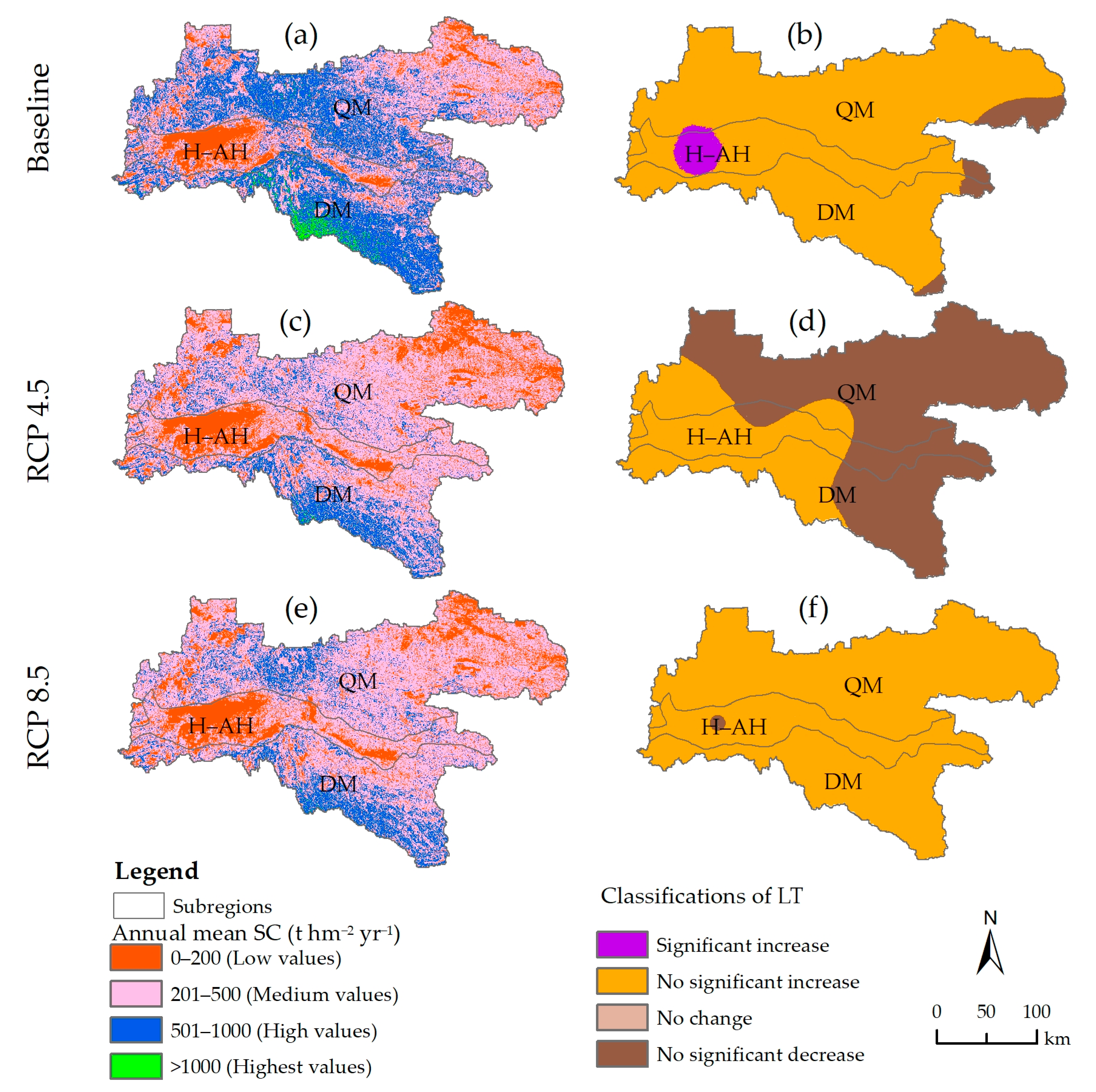
3.1. Spatio-Temporal Variations in SC

The ecological quality in the UHRB has been gradually enhanced by the implementation of the “Grain for Green” project and the Ecological Construction of Protection Forestry in the upstream reaches of the Yangtze River [26]. The resulting revegetation facilitated a significant increase in soil and water ecosystem services [34]. The annual mean SC in the UHRB was 439.72 t hm⁻² yr⁻¹ and the annual SC was slightly enhanced (p > 0.05), ranging across the study area, accounting for 91.79% (Figure 2b) under current climatic conditions (between 2000 and 2015). The annual mean SC was higher overall in the QM and DM highlands that were covered by forest than the grassland and H–AH lowlands, where cropland, wetland, settlement, and unused land were occupied (Figure 2a). Areas of medium SC were aggregated in the northern and southern QM and DM, accounting for 46.8%, followed by the high-value area (35.58%), which was located in the center of the QM and the southern DM. The medium and high SC areas were centered at high altitudes and characterized by forest, while the low SC areas were widespread in the H–AH valley basin area and were covered by wetland and cropland.

The spatial pattern of the annual mean SC under both RCPs was consistent with that under current climate conditions (Figure 2). The linear correlation of the annual mean SC and precipitation was significantly positive across the study region, with the area proportion over 90% under the two RCPs (Figure S1). The projected annual mean SC would respectively be 321.69 t hm⁻² yr⁻¹ and 329.99 t hm⁻² yr⁻¹ under RCP 4.5 and RCP 8.5 in 2030–2045, decreasing by 26.84% and 24.95%, compared to baseline. This was possibly due to the decreased future annual precipitation, which was expected to be −0.09% under RCP 4.5 and −8.69% under RCP 8.5 relative to the baseline (Figure S2). Under RCP 4.5, where the annual precipitation showed a slightly decreasing trend (p > 0.05) (Figure S2), the future annual SC also declined (p > 0.05) by 68.61% (Figure 2); specifically, the high SC was reduced by 60.16%, except in the southeastern zone of the UHRB where SC showed a rising trend, which was reflected in the growth of the low- and medium-service value. Under RCP 8.5, the spatio-temporal pattern of the annual precipitation showed an insignificant increasing trend throughout the study area, where the projected annual SC also increased (p > 0.05) (Figure 2) by 72.41%, while the high SC provision was reduced by 55.93%. The areas showing an increasing trend in value were in the low and medium SC areas, which did not prevent the likely decline in the annual mean service value under RCP 8.5 in comparison to current conditions.

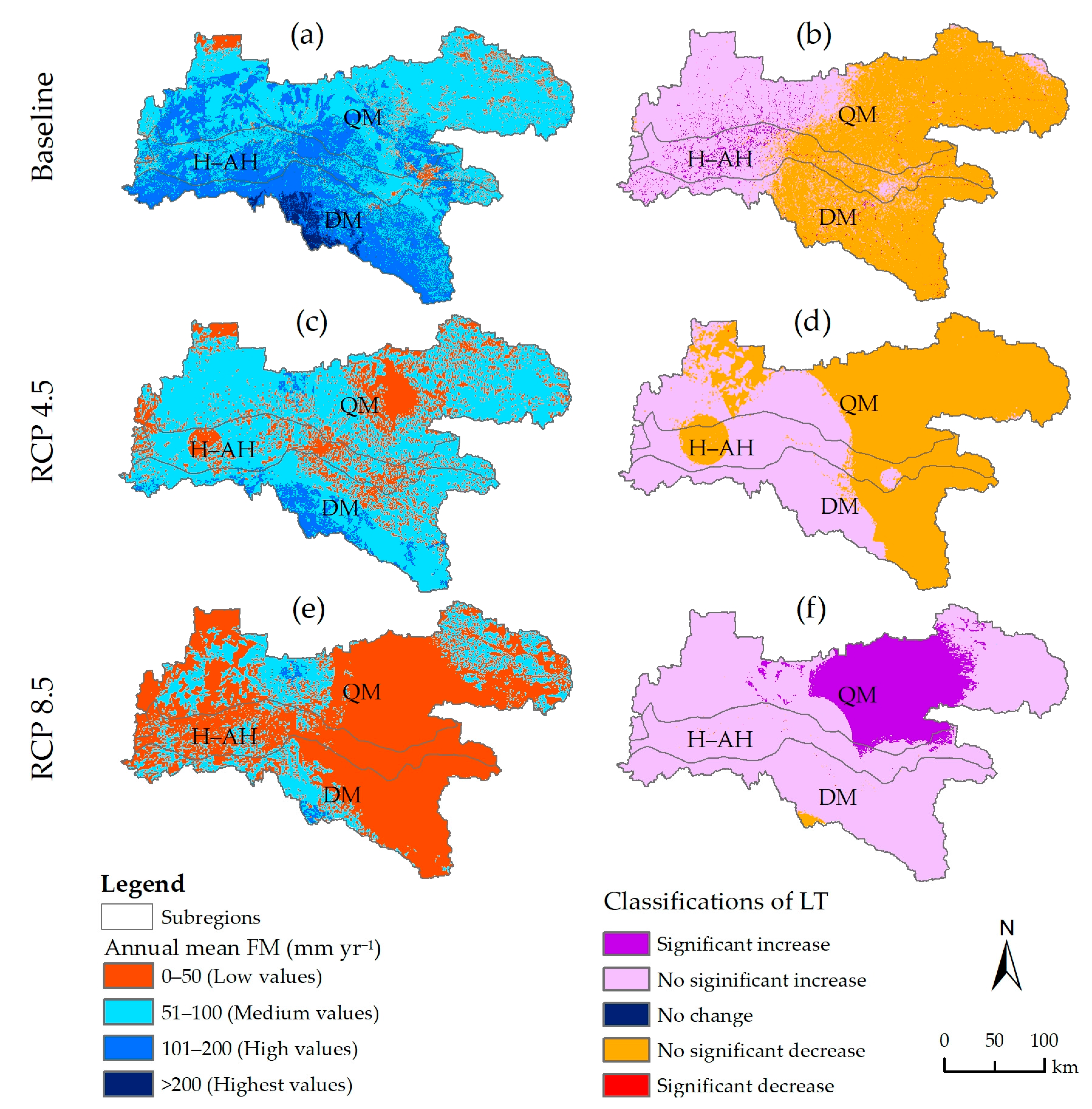
3.2. Spatio-Temporal Variations in FM

The surface runoff was simulated by the water balance algorithm to estimate the flood mitigation service. The annual mean surface runoff was 41.44 mm per year under the baseline and the runoff in the central and the southern UHRB was greater than the other areas (Figure 3). The projected runoff is expected to decrease under the future climate scenarios, with a runoff of 25.29 mm yr⁻¹ and 15.81 mm yr⁻¹ under RCP 4.5 and RCP 8.5, respectively. The linear correlation showed that the annual runoff and rainstorm events had significant positive inter-relationships under the two RCPs (98.36% and 96.18%, respectively) (Figure S3). The linear trend in the annual runoff under future climate scenarios registered a spatio-temporal change in future rainstorms (Figure S4). The projected runoff was simulated to decrease by 38.96% and 61.84%, with a reduction of 34.99% and 59.17% in annual mean rainstorms, respectively, under the two RCPs compared to the baseline. Under RCP 4.5, rainstorm events decreased (p > 0.05) in the eastern part of the UHRB, where the runoff also decreased with a non-significant trend (57.80%). Rainstorm events increased (p > 0.05) in the eastern part of the UHRB, where the runoff also increased with a non-significant trend (40.69%). Under RCP 8.5, the annual runoff and rainstorm frequency had an increasing trend overall: when the rainstorms increased (p < 0.05), the annual runoff grew with a significant trend (accounting for 38.40%), and when the rainstorms rose with a non-significant trend, the annual runoff grew non-significantly (accounting for 58.09%). However, the annual mean values for both were lower than those under present conditions.

The annual mean FM for the baseline was 98.36 mm yr⁻¹ and showed a slightly increasing trend between 2000 to 2015. The annual mean FM was relatively high in the northern and southern UHRB, which was characterized by a high altitude and forest (Figure 1), compared to other regions during the same period (Figure 4a). The largest area (57.78%) had a medium level of service distributed at moderate elevations with a large area of grassland, including the central and northeastern QM and the westernH–AH. High FM (35.05%) was present in the western and southern QM and DM.

The spatial distribution of annual mean FM under the two RCPs can be found in the pattern of that under baseline (Figure 4c,e). The annual mean FM was projected to decrease by approximately 34.12% and 58.56%, following a decline of 34.99% and 59.17% in annual mean rainstorm projections under RCP 4.5 and RCP 8.5, respectively, when compared to the baseline. Medium and low FM will cover a large proportion in the entire study area under RCP 4.5 and RCP 8.5, respectively. The linear correlation of annual mean FM and rainstorm was significantly positive under future climate change throughout the whole study area (Figure S5). Patterns of the linear trend change in FM projections (Figure 4) also reflected the projected rainstorm changes from 2030 to 2045 (Figure S4). Under RCP 4.5, where the rainstorm projections showed an increase (p > 0.05), the annual FM will increase (p > 0.05) by a total of 53.09% in low and medium service areas, while the FM will decrease (p > 0.05) by 88.45% in high service areas with non-significant rainstorm declines compared to present conditions. Under RCP 8.5, the increased rainstorms will result in growing FM, with a total of 58.63% in low and medium service areas. We also found that the low service areas were the areas of noticeable change with significant increasing trends. The low FM in this scenario will account for 72.06% of the study area, which indicated that the flood mitigation capacity overall will be apparently lower than that between 2000–2015 and under RCP 4.5.

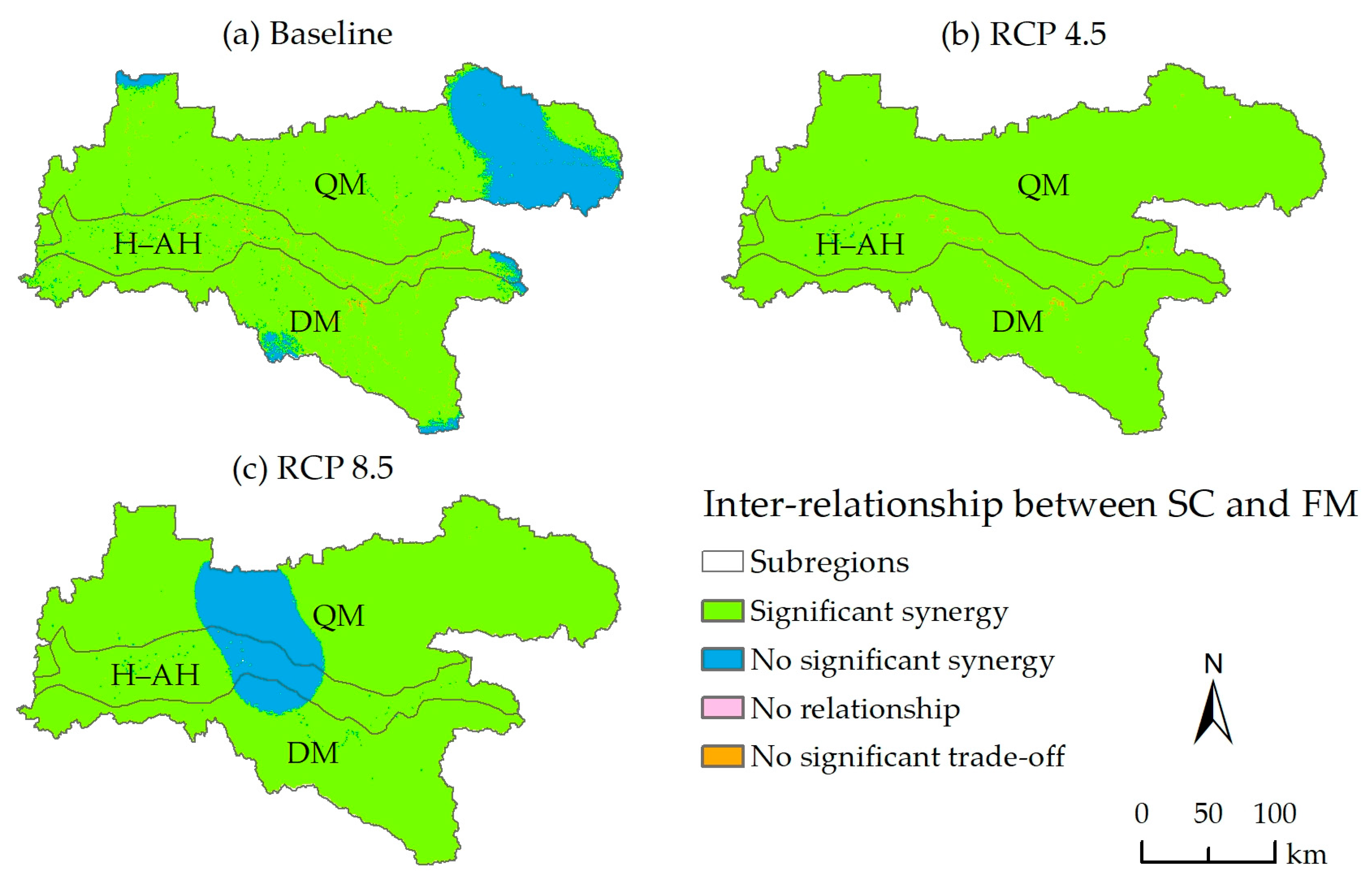
3.3. Spatial Heterogeneity in the Inter-Relationship between SC and FM

The inter-relationship between SC and FM varied across different regions for the baseline (Figure 5a). Generally, it showed a synergistic pattern and the area of significant synergies (p ≤ 0.05) covered 85.61% of the UHRB. These areas were aggregated in the western and middle QM (42.36%), the northern and central DM (25.95%), and the H–AH (17.3%) subregions.

We then examined the inter-relationship of two ESs for 2030–2045 and the significant synergy between SC and FM will be enhanced by 16.48% and 2.95% under RCP4.5 and RCP 8.5 against the baseline, respectively, in the UHRB (Figure 5b,c). The dominant inter-relationship between SC and FM under RCP 4.5 was synergistic at a significant level, accounting for 99.72% of the UHRB. A similar inter-relationship pattern resulted under RCP 8.5, where the area proportions of the inter-relationship at significant and insignificant grades were 88.14% and 11.81%, respectively. The areas with a synergetic relationship at an insignificant level will shift from the northeast to the northwest of the UHRB under RCP 8.5. Overall, a synergistic inter-relationship between SC and FM was observed for all three future scenarios, with the synergistic relationship expected to increase under RCP 4.5 and RCP 8.5. Predicted changes in the climate could enhance the inter-relationship between SC and FM services across the UHRB.

4. Discussion

The changing precipitation as a consequence of changing climatic conditions in the UHRB is the main determinant of the ESs supply, where the changing trend in precipitation directly shows the magnitude of the corresponding changing ESs. This has also been found in ecosystem service and climate-related research in southern California [2] and the Gandheswari watershed in eastern India [17]. More recently, scientists have projected decreasing precipitation in southern Europe, and the same outcome was shown in this study; however, precipitation will grow in most areas of northern Europe [59].

Analyzing the impact of climate change on ESs and the inter-relationships between ESs in the near term may provide a timely scientific basis for policy design and formulating climate adaptation strategies. Our study indicated that the SC and FM supply will decrease along with the reduced precipitation and rainstorms in the UHRB under the two RCPs, further indicating that ecosystem resilience will be weakened and the regulation of soil and water services will be reduced from 2030 to 2045. That is, the changing climate conditions will exert pressure on the ability of the ecosystem to provide benefits for human beings, leading to resource losses, as well as ecological deterioration [64]. The degradation of ecosystem services exacerbates soil erosion and desertification [65,66], seriously affects food safety, and directly threatens regional ecological security [67,68]. Furthermore, as the water source for the middle route of the S–NWDP, the ecological degradation of the UHRB will reduce soil retention and result in water quality deterioration for the middle and downstream reaches of the UHRB and the beneficiaries of the middle line of the S–NWDP [28,33]. In order to ensure that water quality will be maintained for the middle line of the S–NWDP, the cost of water purification and infrastructure may increase in the future.

Considering the impact of changing climatic conditions on the inter-relationship between ESs is an important innovation in ES research. The governing of trade-offs and synergies is known to reinforce the resilience of ecosystems, consequently improving the ability of ecosystems to benefit human beings [5,8]. The results from this study indicated that the synergistic inter-relationship between SC and FM will be enhanced in the period 2030–2045. The inter-relationships between services are largely conditional on social and economic development [69], and trade-offs and synergies can switch through ecosystem regime shifts [5]. Strategies aimed at promoting socio-economic development should consider balancing resource exploitation and ecosystem sustainability given the crucial role ES inter-relationships play in ecologically sustainable development [5,8].

The findings of this study demonstrated that surface runoff will decrease under future climate scenarios, becoming worse under RCP 8.5. The decreasing runoff will not only inevitably affect water demand from the water diversion project but also influence urban water supplies, agricultural irrigation, and shipping traffic in the middle and lower reaches of the Hanjiang River, changing the erosion and siltation conditions in the river and reducing the self-regulating capacity of the river due to hydrological variations [33,64]. Studies have shown that the spatial distribution of crops across the landscape is subject to local climatic conditions (e.g., rainfall) [34]. Stakeholders are concerned about the efficacy of easing the negative stress from climate variability through land-use change [59]. This would result in changes in cropland management, such as an adjustment in farming patterns [59] and drought-tolerant crops planting, which can mitigate the vulnerability and increase the resilience to changed climate conditions [70] in the Hanjiang River Basin.

The operation of the middle line of the water transfer project has altered the Hanjiang river flow rate and consequently influenced the water quality since the water purification capacity of the middle and downstream river reaches would probably be reduced due to decreased inflow [71]. Moreover, Kuo [71] found that the flow rate in the middle and downstream end of the Hanjiang River should be raised in order to prevent water quality deterioration and effectively deal with pollutants. However, this would be a great challenge since the annual precipitation and runoff in the UHRB will be greatly reduced under future scenarios.

Our study on the potential impacts of future climates on SC and FM services and their inter-relationship in the UHRB provided evidence for integrating climate change into the designation of ecological conservation of watersheds. The management of landscapes for biological conservation and ecologically sustainable natural resource use are crucial global issues. Understanding the inter-relationships of soil and water conservation services can help with ecosystem resources management and improve the ratio of resource utilization [53,59]. More recently, it has been confirmed that 5.47% of the discharge areas in the UHRB have been identified as high priorities based on water–soil conservation [72] but this did not take into account climate change. Furthermore, the UHRB is in a highly forested river basin, and given the crucial role of forests in mitigation of changing climates, especially in carbon sequestration, climate adaptation strategies should be considered in forestry policies for ecological management [21]. Additionally, it is also imperative to incorporate climate-related policies into ecological environmental management and ecological reserve optimization policy initiatives, such as functional zonation and ecological red lines [2,73] since multiple ESs can be produced in protected areas [74]. Given the impacts of climate change on the ecosystem service inter-relationship, policies can be designed to optimize the synergies between SC and FM services for socio-economic benefits.

The simulation results of the models could not be calibrated effectively due to the scarcity of adequate measurement data; however, the revised universal soil loss equation (RUSLE) and the soil conservation service curve number (SCS-CN) model have been demonstrated to be effective for evaluating the soil conservation service in the UHRB [33,75] and middle and lower reaches of Hanjiang River basin, respectively, and the flood mitigation service in the UHRB [34] and the upper Yangtze River basin [35]. The statistical downscaling method was developed by Liu and Zuo [54] based on the improved stochastic WGEN [55]. Furthermore, the WGEN model we employed to gain daily and specific site climate data was used on the basis of the comparison between the observed and downscaled climate variables [54]. The overall mean confidence interval of parameters and the observed climate mean, as well as the maximum values, were 0.08 and 0.11, respectively, resulting in very high confidence in downscaling future monthly climate variables with reliable parameters. The principal criteria for the procedure were downscaled daily outputs that were consistent with monthly climate projections, both in terms of monthly means and totals. The theoretical framework and approach employed in this study could also be applicable in researching soil sediment, water conservation and purification, the estimation of water yield, etc., in the watersheds, and are also applicable in key natural reserves, biodiversity hotpots, and the water source reserves that are significantly affected by climate conditions.

Some limitations exist in this study. Given that the UHRB is located in the Qinling–Daba mountains, where about 80% of the area is covered by natural vegetation on steep slopes and the land use in this region changed slightly between 2000 and 2014 [34], we assumed that the land-use patterns will stay the same from 2030 to 2045; as such, we only stressed the effects of climate factors on the supply of ecosystem services. However, the change and evolution of the ecosystem structure and environment is a complex process, which is driven by a variety of factors, including socio-economic factors, policy elements, and human’s actual demands of resources [8]. In addition, different climate scenarios can cause different changes in the LULC, followed by the changes in the quality of vegetation coverage and the water–soil regime, resulting in the alteration of soil parameters and the change of the soil water retention capacity [76]. Eventually this changes the quantity and pattern of ESs provision, especially in SC and FM, and their inter-relationship [15]. Moreover, the ESs simulation in this study was a basic step for the comprehensive assessment of the ecosystem service, where the biophysical values of the ESs were not extended to the determination of economic values, which can link ecosystem services to the development of human society and inform economic and environmental policy [21]. Various patterns of trade-offs and synergies are presented based on different scales [6,8]; however, we did not take the spatio-temporal scale dependency of the ecosystem services inter-relationships into account in the study, which may reduce the accuracy of our inter-relationship assessment. The major limitation of our study was that we only selected one GCM model (BNU-ESM) to represent future climate projections. The climate system is a complex construct and the future climate conditions generated from different GCMs vary, resulting in great differences, especially in seasonal precipitation [77]. Previous studies have shown that using multiple GCMs under different emission scenarios is better for providing more robust climate projections [78]. Therefore, multiple GCMs that are downscaled by different methods (e.g., statistical downscaling and dynamical downscaling) under different emission scenarios should be applied to better assess the development of ESs in the future. Despite the above limitations and due to the uniqueness of the East Asian climate, the findings and the scenarios of the CMIP 5 BNU-GCM employed in this study can still provide a framework for understanding the ESs and their inter-relationships and the future consequences for core water supplies. Given the uncertainties of climate change, our next step is to explore multi-model ensemble climate projections with an integrated land–climate model at a high resolution and introduce multiple critical factors (i.e., shared socioeconomic pathways in the scenario framework) of ESs to understand the potential impacts of climate change and other dynamics on ESs and to derive more information to maintain regional and global ecological sustainability.

5. Conclusions

The responses of SC and FM service supplies and their inter-relationship to climate change in the UHRB were assessed by using two future climate scenarios and soil–water conservation models (RUSLE and SCS-CN). The decrease in the provision of SC and FM under the emissions pathways examined with a reduction in precipitation from 2030 to 2045 indicated a reduction in the capacity of the regulating services, which will reduce the ecosystem resilience and result in ecological degradation. The declines in surface runoff in this study were a result of water scarcity increases between 2030 and 2045. The findings above may have serious impacts on human beings in the middle and lower reaches of the Hanjiang river basin and the economic viability of the S–NWDP. Therefore, the potential effects of climate change should be integrated with ecological resource management policies, such as the adjustment of farming patterns and the planting of drought-tolerant crops in land use management, which can be employed to maintain the sustainable development of the river basin. Our results point to regional ecosystem management and climate-related adaptation policy packages for stakeholders to mitigate the negative stress that climate variability will trigger for human welfare and water infrastructure investment.

References

1. Asmus, M.L.; Nicolodi, J.; Anello, L.S.; Gianuca, K. The risk to lose ecosystem services due to climate change: A South American case. Ecol. Eng. 2019, 130, 233–241. [Google Scholar] [CrossRef]
2. Underwood, E.C.; Hollander, A.D.; Safford, H.D.; Kim, J.B.; Srivastava, L.; Drapek, R.J. The impacts of climate change on ecosystem services in southern California. Ecosyst. Serv. 2019, 39, 101008. [Google Scholar] [CrossRef]
3. EEA The European Environment-State and Outlook 2015: European Briefings-Biodiversity. State of the Environment Report; European Environment Agency: Copenhagen, Denmark, 2015.
4. Cristal, I.; Ameztegui, A.; González-Olabarria, J.R.; Garcia-Gonzalo, J. A Decision Support Tool for Assessing the Impact of Climate Change on Multiple Ecosystem Services. Forests 2019, 10, 440. [Google Scholar] [CrossRef] [Green Version]
5. Bennett, E.M.; Peterson, G.D.; Gordon, L.J. Underst. relationships among multiple ecosystem services: Relationships among multiple ecosystem services. Ecol. Lett. 2009, 12, 1394–1404. [Google Scholar] [CrossRef]
6. Hou, Y.; Lü, Y.; Chen, W.; Fu, B. Temporal variation and spatial scale dependency of ecosystem service interactions: A case study on the central Loess Plateau of China. Landsc. Ecol. Dordr. 2017, 32, 1201–1217. [Google Scholar] [CrossRef]
7. Howe, C.; Suich, H.; Vira, B.; Mace, G.M. Creating win-wins from trade-offs? Ecosystem services for human well-being: A meta-analysis of ecosystem service trade-offs and synergies in the real world. Glob. Environ. Chang. 2014, 28, 263–275. [Google Scholar] [CrossRef] [Green Version]
8. Qiao, X.; Gu, Y.; Zou, C.; Xu, D.; Wang, L.; Ye, X.; Yang, Y.; Huang, X. Temporal variation and spatial scale dependency of the trade-offs and synergies among multiple ecosystem services in the Taihu Lake Basin of China. Sci. Total Environ. 2019, 651, 218–229. [Google Scholar] [CrossRef]
9. Hughes, T.P.; Rodrigues, M.J.; Bellwood, D.R.; Ceccarelli, D.; Hoegh-Guldberg, O.; McCook, L.; Moltschaniwskyj, N.; Pratchett, M.S.; Steneck, R.S.; Willis, B. Phase shifts, herbivory, and the resilience of coral reefs to climate change. Curr. Biol. 2007, 17, 360–365. [Google Scholar] [CrossRef] [Green Version]
10. Altieri, M.A. The ecological role of biodiversity in agroecosystems. In Invertebrate Biodiversity as Bioindicators of Sustainable Landscapes; Elsevier: Amsterdam, The Netherlands, 1999; pp. 19–31. [Google Scholar]
11. Clerici, N.; Cote-Navarro, F.; Escobedo, F.J.; Rubiano, K.; Villegas, J.C. Spatio-temporal and cumulative effects of land use-land cover and climate change on two ecosystem services in the Colombian Andes. Sci. Total Environ. 2019, 685, 1181–1192. [Google Scholar] [CrossRef]
12. Tsvetkova, O.; Randhir, T.O. Spatial and temporal uncertainty in climatic impacts on watershed systems. Sci. Total Environ. 2019, 687, 618–633. [Google Scholar] [CrossRef]
13. Ekness, P.; Randhir, T.O. Effect of climate and land cover changes on watershed runoff: A multivariate assessment for storm water management. J. Geophys. Res. Biogeosci. 2015, 120, 1785–1796. [Google Scholar] [CrossRef]
14. Huntington, T.G. Evidence for intensification of the global water cycle: Review and synthesis. J. Hydrol. 2006, 319, 83–95. [Google Scholar] [CrossRef]
15. Liu, Y.; Bi, J.; Lv, J.; Ma, Z.; Wang, C. Spatial multi-scale relationships of ecosystem services: A case study using a geostatistical methodology. Sci. Rep. 2017, 7, 1–12. [Google Scholar] [CrossRef] [PubMed] [Green Version]
16. Sharp, R.; Chaplin-Kramer, R.; Wood, S.; Guerry, A.; Tallis, H.; Ricketts, T.; Nelson, E.; Ennaanay, D.; Wolny, S.; Olwero, N.; et al. InVEST User’s Guide; The Natural Capital Project, Stanford University, University of Minnesota, The Nature Conservancy, and World Wildlife Fund, 2018; Available online: http://data.naturalcapitalproject.org/nightly-build/release_default/rele (accessed on 10 September 2019).
17. Pal, S.C.; Chakrabortty, R. Simulating the impact of climate change on soil erosion in sub-tropical monsoon dominated watershed based on RUSLE, SCS runoff and MIROC5 climatic model. Adv. Space Res. 2019, 64, 352–377. [Google Scholar] [CrossRef]
18. Roy, P. Application of USLE in a GIS environment to estimate soil erosion in the Irga watershed, Jharkhand, India. Phys. Geogr. 2019, 40, 361–383. [Google Scholar] [CrossRef]
19. Kattel, G.R.; Shang, W.; Wang, Z.; Langford, J. China’s South-to-North Water Diversion Project Empowers Sustainable Water Resources System in the North. Sustainability 2019, 11, 3735. [Google Scholar] [CrossRef] [Green Version]
20. Mortoja, M.G.; Yigitcanlar, T. Local Drivers of Anthropogenic Climate Change: Quantifying the Impact through a Remote Sensing Approach in Brisbane. Remote Sens. 2020, 12, 2270. [Google Scholar] [CrossRef]
21. Ding, H.; Chiabai, A.; Silvestri, S.; Nunes, P.A.L.D. Valuing climate change impacts on European forest ecosystems. Ecosyst. Serv. 2016, 18, 141–153. [Google Scholar] [CrossRef]
22. Waongo, M.; Laux, P.; Kunstmann, H. Adaptation to climate change: The impacts of optimized planting dates on attainable maize yields under rainfed conditions in Burkina Faso. Agric. For. Meteorol. 2015, 205, 23–39. [Google Scholar] [CrossRef] [Green Version]
23. Albrich, K.; Rammer, W.; Thom, D.; Seidl, R. Trade-offs between temporal stability and level of forest ecosystem services provisioning under climate change. Ecol. Appl. 2018, 28, 1884–1896. [Google Scholar] [CrossRef] [Green Version]
24. Markkula, I.; Turunen, M.; Rasmus, S. A review of climate change impacts on the ecosystem services in the Saami Homeland in Finland. Sci. Total Environ. 2019, 692, 1070–1085. [Google Scholar] [CrossRef]
25. Runting, R.K.; Bryan, B.A.; Dee, L.E.; Maseyk, F.J.F.; Mandle, L.; Hamel, P.; Wilson, K.A.; Yetka, K.; Possingham, H.P.; Rhodes, J.R. Incorporating climate change into ecosystem service assessments and decisions: A review. Glob. Chang. Biol. 2017, 23, 28–41. [Google Scholar] [CrossRef] [Green Version]
26. Gong, J.; Liu, D.; Zhang, J.; Xie, Y.; Cao, E.; Li, H. Tradeoffs/synergies of multiple ecosystem services based on land use simulation in a mountain-basin area, western China. Ecol. Indic. 2019, 99, 283–293. [Google Scholar] [CrossRef]
27. Civantos, E.; Thuiller, W.; Maiorano, L.; Guisan, A.; Araújo, M.B. Potential Impacts of Climate Change on Ecosystem Services in Europe: The Case of Pest Control by Vertebrates. BioScience 2012, 62, 658–666. [Google Scholar] [CrossRef] [Green Version]
28. Han, B.; Meng, N.; Zhang, J.; Cai, W.; Wu, T.; Kong, L.; Ouyang, Z. Assessment and Management of Pressure on Water Quality Protection along the Middle Route of the South-to-North Water Diversion Project. Sustainability 2019, 11, 3087. [Google Scholar] [CrossRef] [Green Version]
29. Zhu, Y.P.; Zhang, H.P.; Chen, L.; Zhao, J.F. Influence of the South–North Water Diversion Project and the mitigation projects on the water quality of Han River. Sci. Total Environ. 2008, 406, 57–68. [Google Scholar] [CrossRef]
30. Zhao, Z.; Yan, S.; Tong, Y.; Wei, Y. Eco-environmental Status Assessment and Countermeasures in the Upper Hanjiang River Basin. Bull. Soil Water Conserv. 2012, 32, 32–60. (In Chinese) [Google Scholar] [CrossRef]
31. Dong, M.; Tang, M.; Li, S.; Cao, H.; Deng, H.; Wu, G. Effects of water transfer project construction on vegetation patterns. Acta Ecol. Sin. 2016, 36, 6656–6663. (In Chinese) [Google Scholar] [CrossRef]
32. Guo, H.; Liu, R.; He, X.; Tian, Z. Eco-environmental evaluation of Middle Route of South-to-North Transfer Project based on PSR model. South-North Water Transf. Water Sci. Technol. 2017, 15, 65–70. (In Chinese) [Google Scholar] [CrossRef]
33. Li, X.; Wang, Z. Evaluation of soil loss and ecological benefit in the Han river source. Resour. Environ. Yangtze Basin 2016, 25, 671–678. (In Chinese) [Google Scholar] [CrossRef]
34. Wang, P.; Zhang, L.; Li, Y.; Jiao, L.; Wang, H.; Yan, J.; Lü, Y.; Fu, B. Spatio-temporal variations of the flood mitigation service of ecosystem under different climate scenarios in the Upper Reaches of Hanjiang River Basin, China. J. Geogr. Sci. 2018, 28, 1385–1398. [Google Scholar] [CrossRef] [Green Version]
35. Fu, B.; Wang, Y.K.; Xu, P.; Yan, K. Mapping the flood mitigation services of ecosystems – A case study in the Upper Yangtze River Basin. Ecol. Eng. 2013, 52, 238–246. [Google Scholar] [CrossRef]
36. Baró, F.; Haase, D.; Gómez-Baggethun, E.; Frantzeskaki, N. Mismatches between ecosystem services supply and demand in urban areas: A quantitative assessment in five European cities. Ecol. Indic. 2015, 55, 146–158. [Google Scholar] [CrossRef] [Green Version]
37. Rao, E.; Ouyang, Z.; Yu, X.; Xiao, Y. Spatial patterns and impacts of soil conservation service in China. Geomorphology 2014, 207, 64–70. [Google Scholar] [CrossRef]
38. Wischmeier, W.H.; Smith, D.D. Predicting Rainfall Erosion Losses—A Guide to Conservation Planning; No. 537; Science, US Department of Agriculture Handbook: Washington, DC, USA, 1978.
39. Sharpley, A.N.; Williams, J.R. EPIC-erosion/productivity impact calculator: 1. Model Doc. 1990. [Google Scholar]
40. McCool, D.K.; Brown, L.C.; Foster, G.R.; Mutchler, C.K.; Meyer, L.D. Revised slope steepness factor for the Universal Soil Loss Equation. Trans. ASAE 1987, 30, 1387–1396. [Google Scholar] [CrossRef]
41. Cai, C.; Ding, S.; Shi, Z.; Huang, L.; Zhang, G. Study of Applying USLE and Geographical Information System IDRISI to Predict Soil Erosion in Small Watershed. J. Soil Water Conserv. 2000, 14, 19–24. (In Chinese) [Google Scholar]
42. Fu, B.; Liu, Y.; Lü, Y.; He, C.; Zeng, Y.; Wu, B. Assessing the soil erosion control service of ecosystems change in the Loess Plateau of China. Ecol. Complex. 2011, 8, 284–293. [Google Scholar] [CrossRef]
43. Lufafa, A.; Tenywa, M.M.; Isabirye, M.; Majaliwa, M.J.G.; Woomer, P.L. Prediction of soil erosion in a Lake Victoria basin catchment using a GIS-based Universal Soil Loss model. Agric. Syst. 2003, 76, 883–894. [Google Scholar] [CrossRef]
44. Bhuyan, S.J.; Mankin, K.R.; Koelliker, J.K. Watershed–Scale amc Selection for Hydrologic modeling. Trans. ASAE 2003, 46, 8. [Google Scholar] [CrossRef]
45. Mishra, S.K.; Pandey, A.; Singh Vijay, P. Special Issue on Soil Conservation Service Curve Number (SCS-CN) Methodology. J. Hydrol. Eng. 2012, 17, 1157. [Google Scholar] [CrossRef]
46. Hooshyar, M.; Wang, D. An analytical solution of Richards’ equation providing the physical basis of SCS curve number method and its proportionality relationship. Water Resour. Res. 2016, 52, 6611–6620. [Google Scholar] [CrossRef]
47. Mishra, S.K.; Singh, V.P. (Eds.) SCS-CN Method. In Soil Conservation Service Curve Number (SCS-CN) Methodology; Water Science and Technology Library; Springer: Dordrecht, The Netherlands, 2003; pp. 84–146. ISBN 978-94-017-0147-1. [Google Scholar]
48. Soil Conservation Service. National Engineering Handbook, Section 4: Hydrology; US Soil Conservation Service, USDA: Washington, DC, USA, 1985.
49. Cameron, S. Making Regression Analysis More Useful, II. Econom. Maidenhead Mcgraw Hill High. Educ. 2005, 171–198. Available online: https://www.thecasecentre.org/educators/products/view?&id=92081 (accessed on 20 September 2020).
50. Lü, Y.; Zhang, L.; Feng, X.; Zeng, Y.; Fu, B.; Yao, X.; Li, J.; Wu, B. Recent ecological transitions in China: Greening, browning, and influential factors. Sci. Rep. 2015, 5, 8732. [Google Scholar] [CrossRef]
51. Zheng, H.; Zhang, L.; Wang, P.; Li, Y. The NPP-Based Composite Indicator for Assessing the Variations of Water Provision Services at the National Scale. Water 2019, 11, 1628. [Google Scholar] [CrossRef] [Green Version]
52. Pearson, K.; Galton, F. VII. Note on regression and inheritance in the case of two parents. Proc. R. Soc. Lond. 1895, 58, 240–242. [Google Scholar] [CrossRef]
53. Gutsch, M.; Lasch-Born, P.; Kollas, C.; Suckow, F.; Reyer, C.P.O. Balancing trade-offs between ecosystem services in Germany’s forests under climate change. Environ. Res. Lett. 2018, 13, 045012. [Google Scholar] [CrossRef]
54. Liu, D.L.; Zuo, H. Statistical downscaling of daily climate variables for climate change impact assessment over New South Wales, Australia. Clim. Chang. 2012, 115, 629–666. [Google Scholar] [CrossRef]
55. Richardson, C.W.; Wright, D.A. WGEN: A Model for Generating Daily Weather Variables; U.S. Dept. of Agriculture, Agricultural Research Service; Springfield, National Technical Information Service (NTIS): Washington, DC, USA, 1984.
56. Taylor, K.E.; Stouffer, R.J.; Meehl, G.A. An Overview of CMIP5 and the Experiment Design. Bull. Amer. Meteor. Soc. 2011, 93, 485–498. [Google Scholar] [CrossRef] [Green Version]
57. Thomson, A.M.; Calvin, K.V.; Smith, S.J.; Kyle, G.P.; Volke, A.; Patel, P.; Delgado-Arias, S.; Bond-Lamberty, B.; Wise, M.A.; Clarke, L.E.; et al. RCP4.5: A pathway for stabilization of radiative forcing by 2100. Clim. Chang. 2011, 109, 77. [Google Scholar] [CrossRef] [Green Version]
58. Riahi, K.; Rao, S.; Krey, V.; Cho, C.; Chirkov, V.; Fischer, G.; Kindermann, G.; Nakicenovic, N.; Rafaj, P. RCP 8.5—A scenario of comparatively high greenhouse gas emissions. Clim. Chang. 2011, 109, 33. [Google Scholar] [CrossRef] [Green Version]
59. Schröter, D.; Cramer, W.; Leemans, R.; Prentice, I.C.; Araújo, M.B.; Arnell, N.W.; Bondeau, A.; Bugmann, H.; Carter, T.R.; Gracia, C.A.; et al. Ecosystem Service Supply and Vulnerability to Global Change in Europe. Science 2005, 310, 1333–1337. [Google Scholar] [CrossRef] [PubMed] [Green Version]
60. Fischer, G.; Nachtergaele, F.; Prieler, S.; Van Velthuizen, H.T.; Verelst, L.; Wiberg, D. Global Agro-Ecological Zones Assessment for Agriculture (GAEZ 2008); IIASA: Laxenburg Austria; FAO: Rome, Italy, 2008. [Google Scholar]
61. Li, Y.; Zhang, L.; Qiu, J.; Yan, J.; Wan, L.; Wang, P.; Hu, N.; Cheng, W.; Fu, B. Spatially explicit quantification of the interactions among ecosystem services. Landsc. Ecol. 2017, 32, 1181–1199. [Google Scholar] [CrossRef]
62. Wang, J.; Lü, Y.; Zeng, Y.; Zhao, Z.; Zhang, L.; Fu, B. Spatial heterogeneous response of land use and landscape functions to ecological restoration: The case of the Chinese loess hilly region. Environ. Earth Sci. 2014, 72, 2683–2696. [Google Scholar] [CrossRef] [Green Version]
63. Zhang, L.; Fu, B.; Lü, Y.; Zeng, Y. Balancing multiple ecosystem services in conservation priority setting. Landsc. Ecol. 2015, 30, 535–546. [Google Scholar] [CrossRef]
64. Liu, H.; Wu, J.; Liao, M. Ecosystem service trade-offs upstream and downstream of a dam: A case study of the Danjiangkou dam, China. Arab J. Geosci. 2019, 12, 17. [Google Scholar] [CrossRef] [Green Version]
65. Lang, Y.; Song, W. Quantifying and mapping the responses of selected ecosystem services to projected land use changes. Ecol. Indic. 2019, 102, 186–198. [Google Scholar] [CrossRef]
66. Vaezi, A.R.; Ahmadi, M.; Cerdà, A. Contribution of raindrop impact to the change of soil physical properties and water erosion under semi-arid rainfalls. Sci. Total Environ. 2017, 583, 382–392. [Google Scholar] [CrossRef]
67. Mingkuan, W.; Hongwei, M. The Impact of Spatial Heterogeneity on Ecosystem Service Value in a Case Study in Liuyang River Basin, China. J. Resour. Ecol. 2018, 9, 209–218. [Google Scholar] [CrossRef]
68. Munns, W.R.; Rea, A.W.; Suter, G.W.; Martin, L.; Blake-Hedges, L.; Crk, T.; Davis, C.; Ferreira, G.; Jordan, S.; Mahoney, M.; et al. Ecosystem services as assessment endpoints for ecological risk assessment. Integr. Environ. Assess. Manag. 2016, 12, 522–528. [Google Scholar] [CrossRef]
69. Briner, S.; Huber, R.; Bebi, P.; Elkin, C.; Schmatz, D.R.; Grêt-Regamey, A. Trade-Offs between Ecosystem Services in a Mountain Region. Ecol. Soc. 2013, 18. [Google Scholar] [CrossRef] [Green Version]
70. He, L.; Cleverly, J.; Wang, B.; Jin, N.; Mi, C.; Liu, D.L.; Yu, Q. Multi-model ensemble projections of future extreme heat stress on rice across southern China. Appl. Clim. 2018, 133, 1107–1118. [Google Scholar] [CrossRef]
71. Kuo, Y.-M.; Liu, W.; Zhao, E.; Li, R.; Munoz-Carpena, R. Water quality variability in the middle and down streams of Han River under the influence of the Middle Route of South-North Water diversion project, China. J. Hydrol. 2019, 569, 218–229. [Google Scholar] [CrossRef]
72. Wu, H. Watershed prioritization in the upper Han River basin for soil and water conservation in the South-to-North Water Transfer Project (middle route) of China. Environ. Sci. Pollut. Res. 2018, 25, 2231–2238. [Google Scholar] [CrossRef]
73. Nelson, E.J.; Kareiva, P.; Ruckelshaus, M.; Arkema, K.; Geller, G.; Girvetz, E.; Goodrich, D.; Matzek, V.; Pinsky, M.; Reid, W.; et al. Climate change’s impact on key ecosystem services and the human well-being they support in the US. Front. Ecol. Environ. 2013, 11, 483–893. [Google Scholar] [CrossRef] [Green Version]
74. Zeng, J.; Chen, T.; Yao, X.; Chen, W. Do Protected Areas Improve Ecosystem Services? A Case Study of Hoh Xil Nature Reserve in Qinghai-Tibetan Plateau. Remote Sens. 2020, 12, 471. [Google Scholar] [CrossRef] [Green Version]
75. Wang, P.; Zhang, L.; Li, Y.; Jiao, L.; Wang, H.; Yan, J.; Lü, Y.; Fu, B. Spatio-temporal characteristics of the trade-off and synergy relationships among multiple ecosystem services in the Upper Reaches of Hanjiang River Basin. Acta Geogr. Sin. 2017, 72, 2064–2078. (In Chinese) [Google Scholar] [CrossRef]
76. Lorencová, E.; Frélichová, J.; Nelson, E.; Vačkář, D. Past and future impacts of land use and climate change on agricultural ecosystem services in the Czech Republic. Land Use Policy 2013, 33, 183–194. [Google Scholar] [CrossRef]
77. Wang, B.; Liu, D.; Asseng, S.; Macadam, I.; Yang, X.; Yu, Q. Spatiotemporal changes in wheat phenology, yield and water use efficiency under the CMIP5 multimodel ensemble projections in eastern Australia. Clim. Res. 2017, 72, 83–99. [Google Scholar] [CrossRef]
78. Tebaldi, C.; Knutti, R. The use of the multi-model ensemble in probabilistic climate projections. Philos. Trans. R. Soc. A Math. Phys. Eng. Sci. 2007, 365, 2053–2075. [Google Scholar] [CrossRef]
Figure 1. Overview of the UHRB (Upper Hanjiang River Basin) in Shaanxi Province. The details are as follows: (a) the location of the Hanjiang River Basin and the UHRB in China, including the surrounding important rivers; (b) the distribution of the 19 meteorological stations and three subregions: QM (Qinling Mountain Region), H–AH (Hanzhong–Ankang Hilly region), and DM (Daba Mountain Region), and the elevation characteristics of the UHRB; (c) the LULC (land-use and land-cover) classifications in the UHRB in 2015.
Water 12 02825 g001
Figure 2. The spatial pattern of annual mean soil conservation (SC) (t hm−2 yr−1) and the significance classifications of the linear trend (LT) of SC for the baseline from 2000 to 2015 and under the two emission Representative Concentration Pathways (RCP 4.5 and RCP 8.5) from 2030 to 2045. (a,c,e) shows the spatial patterns of the annual mean SC for three scenarios, and the size of the value was proportional to the amount of ecosystem services (ESs), that is, the larger the value, the larger the ES, and vice versa. The annual mean SC was categorized into four classes: low values (0–200), medium values (201–500), high values (501–1000), and highest values (>1000). (b,d,f) indicates the significance classifications of the linear trend of the annual SC under the three scenarios.
Water 12 02825 g002
Figure 3. The spatial pattern of the annual mean runoff and the significance classifications of the LT of the runoff for the baseline from 2000 to 2015 and under the two emission pathways (RCP 4.5 and RCP 8.5) from 2030 to 2045. (a,c,e) shows the spatial patterns of the annual mean runoff in the three scenarios, where the annual mean runoff was categorized into four classes: low values (0–50), medium values (51–150), high values (151–250), and highest values (>250). (b,d,f) shows the significance classifications of the linear trend of annual runoff in the three scenarios.
Water 12 02825 g003
Figure 4. The spatial patterns of the annual mean FM (mm yr1) and the significance classifications of the LT of FM for the baseline from 2000 to 2015 and under the two emissions pathways (RCP 4.5 and RCP 8.5) from 2030 to 2045. (a,c,e) indicates the spatial patterns of the annual mean FM under three emissions scenarios, and the size of the value was proportional to the amount of ES. The annual mean FM was categorized into four classes: low values (0–50), medium values (51–100), high values (101–200), and highest values (>200). (b,d,f) indicates the significance of classifications of the LT of annual FM under three emissions scenarios.
Water 12 02825 g004
Figure 5. Inter-relationship of SC and FM under three scenarios, where the significance level here was p ≤ 0.05.
Water 12 02825 g005