Quantile Mixture and Probability Mixture Models in a Multi-Model Approach to Flood Frequency Analysis

Abstract

The classical approach to flood frequency analysis (FFA) may result in significant jumps in the estimates of upper quantiles along with the lengthening series of measurements. Our proposal is a multi-model approach, also called the aggregation technique, which has turned out to be an effective method for the modeling of maximum flows, in large part eliminating the disadvantages of traditional methods. In this article, we present a probability mixture model relying on the aggregation the probabilities of non-exceedance of a constant flow value from the candidate distributions; and we compare it with the previously presented model of quantile mixture, which consists in aggregating the quantiles of the same order from individual models. Here, we defined an asymptotic standard error of design quantiles for both statistical models in two versions: without the bias of quantiles from candidate distributions with respect to aggregated quantiles and with taking it into account. The simulation experiment indicates that the latter version is more accurate and allows for reducing the quantile bias with respect to the unknown population quantile. For the case study, the 0.99 quantiles are determined for both variants of aggregation along with the assessment of its accuracy. The differences between the two proposed aggregation methods are discussed.

1. Introduction

The extreme hydrological phenomena, such as heavy rainfalls, floods, droughts, and storm surges, have been within the interest of scientists for decades. The floods, as the one of natural hazards causing the greatest threat to the life and property of the population and the national economy, are investigated especially now in the days of global climate change [1,2,3,4,5]. Estimating the probable maximum flow in subsequent years is an issue of flood frequency analysis (FFA). According to the principles of hydrological practice, a maximum flow is the greatest instantaneous peak flow of floods in a period of interest, e.g., a hydrological year, season, etc. Maximum flows are determined by the National Hydrological Service by direct measurement of the flow rate in hydrometric profiles on the river. When it is not possible to measure the flow during the culmination (due to dangerous conditions for the measurement teams or too fast hydrological response of the catchment preventing teams from arriving on time), the peak flow is then estimated on the basis of the maximum water level and the current flow rate curve.

In the classical approach to FFA, the procedure involves matching the probability distribution to a series of maximum annual or seasonal flow data and determining for this distribution a quantile of a given (usually high) order. The most commonly used is a quantile of the non-exceedance probability p = 0.99 (x_0.99) , which represents the probable maximum flow that, in stationary conditions, is exceeded on average once in a hundred years [6,7]. The upper quantiles of the distribution of annual maximum flows, called flood quantiles, are design and control characteristics of hydrotechnical structures exposed to high waters or protecting against their negative consequences. Moreover, the upper quantiles are used to determine flood zones and they are the basis for developing strategies to reduce flood risk and loses.

When the annual maxima series is a mixture of winter (snowmelt) and summer (rainfall) flows, a seasonal approach is used [8,9,10,11] that involves the selection of distributions for individual seasons and estimation of their parameters separately. Then, the distribution of annual maxima is determined by means of the selected seasonal distributions. In the case of assuming the independence of the seasonal maximum flows, an annual distribution takes the form of the product model [12,13,14]. Polish hydrological conditions allow for assuming the independence of seasonal peak flows [8,9,15]. However, in the case of dependent seasonal maxima, the distribution of the annual maximum flows can be modeled, for example, using the copula function [15,16]. The seasonal approach is recommended not only because of the genetic heterogeneity of the series of annual maxima for rivers with a mixed thaw-rain flood regime, but an important advantage is that the seasonal approach ensures a logical relationship between seasonal and annual quantiles. The annual quantiles are not smaller than the seasonal quantiles of the same order [17,18].

The true probability distribution of seasonal or annual peak flows is not known; therefore, the choice of the appropriate model distribution and the method of estimating its parameters have always been and still remain the most important decisions in the FFA. In practice, one of the two actions is used: either the adoption of one established probability distribution for all hydrological stations in a given country or region [19,20,21], in particular in Poland [22,23], or the second possible action is the selection of the best distribution from the set of candidate distributions [12,24,25,26] according to the selected discrimination criterion [27,28]. Especially the latter approach may result in significant jumps in the values of the upper quantiles of the distribution along with the lengthening series of measurements. This is the result of changing the parameter values of the current distribution with the incoming new data value, or the result of changing the distribution type, usually from light-tailed to heavy-tailed distribution and the opposite. A classification of distributions commonly used in hydrology with respect to their tail behavior is presented by e.g., Ouarda et al. [29] or El Adlouni et al. [30].

The multi-model approach to FFA proposed by the authors in Bogdanowicz [31] and Markiewicz et al. [32,33], also called aggregation, has turned out to be an effective method of describing the probability distribution of seasonal maximum flows, largely eliminating the disadvantages of traditional methods. The quantile estimates, and thus design values, are much more stable with a growing length of data series than in the case of the classical selection of the best fitted distribution. Markiewicz et al. [33] investigated the problem of the objective selection of models for aggregation; this is of particular importance in the range where the classical FFA reveals a high variability in quantile estimates over the time.

The aim of the study is to extend and improve the aggregation approach proposed so far by the authors by:

• adding a new way of aggregation of distributions—the first variant of aggregation, presented by the authors in [31,32,33], is based on the averaging the values of quantiles of the same order from candidate distributions—here referred to as the mean magnitude (MM) variant. In this paper, it is compared with a new variant of aggregation, named the mean frequency (MF) and based on the averaging over the non-exceedance probabilities (p) of the determined flow value for candidate distributions;
• introducing the analysis of the accuracy of aggregated quantile for both ways of aggregation—so far the analysis of the accuracy of the aggregated quantiles has been a missing element of the aggregation procedure. Here, the analytical form of the asymptotic standard error of aggregated quantile is derived for both aggregation variants. Apart from the classic standard error, its version with the bias of quantiles from candidate distributions relative to the aggregate quantile is also presented.

The paper is organized as follows. After introducing the topic, consequences of the best distribution selection procedure on design in the aspect of growing series of observations are presented in Section 2, i.e., they are significant shifts (visibly unrealistic) in the values of the design quantiles. To mitigate this problem, the authors propose two mixture models, i.e., aggregation of distributions by means of quantiles and by probabilities, defining them in the Methods section. Then, the accuracy of 0.99 quantile in both mixture models, expressed as asymptotic standard error of its estimate, is developed and examined in Section 4. The next section yields the comparison of the properties of both ways of aggregation for the selected case study. Summary and conclusions are given in the last section.

All calculations in this paper were made with the use of Fortran software developed by the authors, repeatedly tested and routinely used in many of our research and study works. The calculations were supported and verified by Excel and Mathematica software.

2. Case Study—Consequences of the Classical Approach to FFA

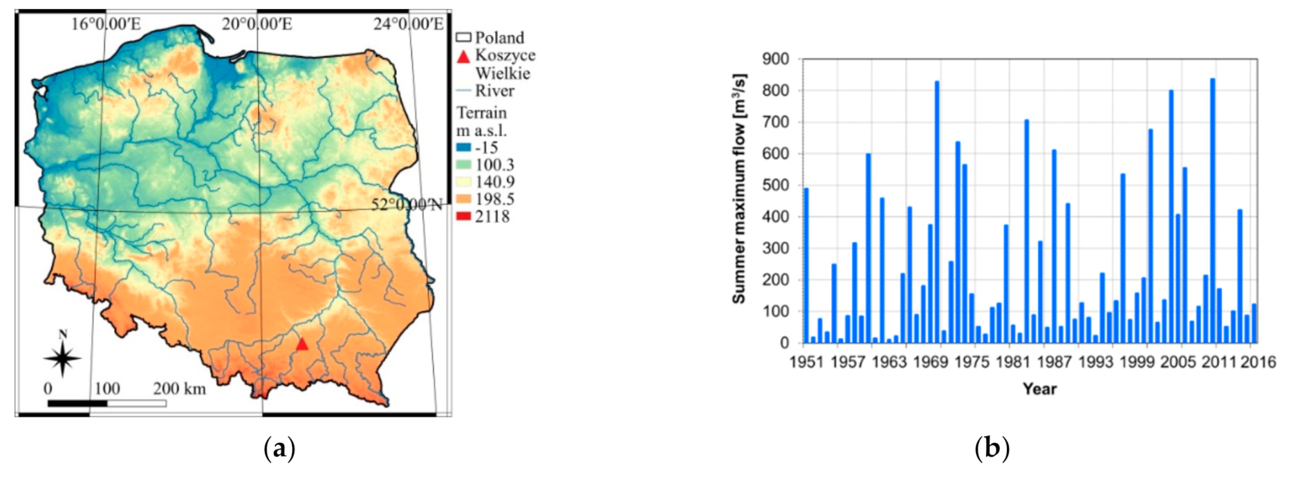
A classical approach to FFA consists of choosing the best probability distribution for describing the data series, in the sense of discrimination criteria, from among hypothetical distributions commonly used for statistical modeling of hydrological extremes. Due to the lack of the knowledge on the true probabilistic model of maximum flows and the limited length of hydrological series, the discussion on the correct choice of the statistical model of maximum flows is unjustified. The criteria of matching a model to empirical data may indicate the best model among the extreme value distributions, but their discrimination power remains low. Moreover, when the length of the series increases (even only by a year), the best model may differ from the one previously selected. Since the best distributions selected in subsequent years of assessment may have different tail thicknesses [30], the estimates of design quantiles can vary significantly from year to year. This problem occurs to a greater or lesser extent for most of the maximum flow data series tested. Here, it is illustrated by the example of the summer maximum flows for the Koszyce Wielkie gauging station on the Biała Tarnowska river, whose hydrological regime is still natural. Biała Tarnowska is located in the south of Poland with the springs on the slopes of Lackowa Mountain between Krynica-Zdrój and Wysowa —right next to the border with Slovakia. Being 105 km long, Biała Tarnowska is the largest right-bank tributary of the Dunajec river (the tributary of the Vistula river) after the Poprad. The basin area of the Biała Tarnowska is 983 km², most of which has a typical mountain character. The slope in the upper reaches is 8.6%, in the lower—about 0.9%. The annual sum of precipitation ranges from about 1000 mm in the upper part of the basin to about 700 in the lower part. The river is characterized by large water level fluctuations (up to 8 m downstream), and sudden summer floods. Rainfall floods in summer (with mean peak flow value of 240 m³/s) dominate winter snowmelt floods (mean peak flow 121 m³/s).

The location of the Koszyce Wielkie station and the observed summer maximum flows from 1951–2016 are shown in Figure 1.

The data consider the period 1951–2016. The calculations have been carried out by gradually lengthening the initial sample 1951–1975 (25 elements) by one year until 2016, so the maximum length of the series is 66 years. For each sample length, the parameters of all five distributions (see

Table 1. Cumulative distribution functions used in the paper.

Distribution	Cumulative Distribution Function (CDF)
Gamma (Ga)	$F\left(x\right)=\frac{\gamma \left[k,\left(x-\epsilon \right)\alpha \right]}{\mathsf{\Gamma }\left(k\right)}$
Weibull (We)	$F\left(x\right)=1-\exp \left[-{\left(\frac{x-\epsilon }{\alpha }\right)}^k\right]$
Inverse Gaussian (IG)	$F\left(x\right)=\frac{1}{2}\left[2-erfc\left(\frac{-\alpha +\left(x-\epsilon \right)k/\alpha }{\sqrt{x-\epsilon }}\right)+\exp \left(4k\right)erfc\left(\frac{\alpha +\left(x-\epsilon \right)k/\alpha }{\sqrt{x-\epsilon }}\right)\right]$
Generalized exponential (GE)	$F\left(x\right)={\left[1-\exp \left(-\alpha x\right)\right]}^k$
Log-normal (LN)	$F(x)=\frac{1}{2}erfc\left(-\frac{In(x)-\alpha }{k\sqrt{2}}\right)$

$\gamma \left[a,b\right]={{\displaystyle \int }}_0^b{z}^{a-1}\exp \left(-z\right)dz$ is the lower incomplete beta function [37] (p. 762); $erfc\left(z\right)=\frac{2}{\sqrt{\pi }}{{\displaystyle \int }}_z^{\infty }\exp \left(-t^2\right)dt$ is the complementary error function [37] (p. 766).

) have been estimated using the maximum likelihood method (MLM) [34]; then, each distribution has been tested by χ² and Kołmogorov–Smirnov goodness of fit tests [35]. Except for only a few cases, all the distributions met both goodness of fit tests for each sample length. The distribution that did not meet the test was removed from current calculation. Finally, the Akaike information criterion (AIC) [36] was used to select the best fitted model among candidates. A variability of the selection of the best distribution along with the related 0.99 quantile for summer maximum flow is depicted in Figure 2 (in black).

Figure 2 shows the quantile sudden rises in the period 1990–2000 associated with the selection of the best distribution that has a heavier tail (IG, LN) than the counter-candidates (Ga, We, GE) [30]. The value of the design quantile nearly doubled. This situation is particularly inconvenient for hydrological information users (e.g., designers, engineers, stakeholders), who expect from hydrologists not only raw statistical analysis results, but also their evaluation and possible correction. Using the aggregation method presented in our previous papers, the 0.99 quantile has been determined for each year of assessment based on a set of five candidate distributions (red line in Figure 2). Note that the aggregate values of design quantile have relatively small fluctuations that are acceptable from a practical point of view. Apart from the two visible peaks, the aggregate quantile values are higher than the quantile values estimated on the basis of the best-matching distribution; this is the result of including light and heavier tail distributions in the analysis. When determining design quantiles, both by selection of the best distribution and by aggregating quantiles, it is particularly important to correctly define the set of candidate distributions (which should meet the goodness of fit tests at first). A set of heavy tailed distributions will result in higher estimates of upper quantiles than in the case of light tailed distributions, equally well matched to the data in the main probability mass for both sets of distributions. Both extremes are undesirable from the point of view of practitioners, engineers. Overstated estimates of design values increase the costs of hydrotechnical investments, and lowered estimates increase the risk of flooding and other damage with the occurrence of large waters.

3. Methods

3.1. Probability Distributions for Modeling of Maximum Flows

For flood frequency modeling, the probability distributions with no upper bound of domain and non-negative skewness are usually used. In this paper, five distributions are investigated: gamma (Ga), Weibull (We), inverse Gaussian (IG), generalized exponential (GE), and log-normal (LN). Their cumulative distribution functions (CDF) are presented in Table 1, where: $\epsilon \ge 0$ is a location parameter, $\alpha >0$ is a scale parameter, $k>0$ is a shape parameter, and random variable $x\ge \epsilon$.

The Ga, We, and LN distributions are commonly used in the FFA, while the IG and GE distributions have been introduced to flood frequency modeling of Polish data by Strupczewski et al. [38] and Markiewicz et al. [32], respectively. As investigated in Markiewicz et al. [32,33], the latter two distributions with the location parameter equal to zero are suitable for modeling of maximum flows for Polish rivers.

3.2. Two Aggregation Schemes

The aggregation of distributions can be done in two ways:

• the aggregation by a mixture of quantile values of the same order obtained from candidate distributions (MM—Mean magnitude), which has been presented in our previous papers [31,32,33].
• the aggregation by a mixture of probability from candidate distributions obtained for fixed quantile value (MF—Mean frequency), which is our new and original proposal.

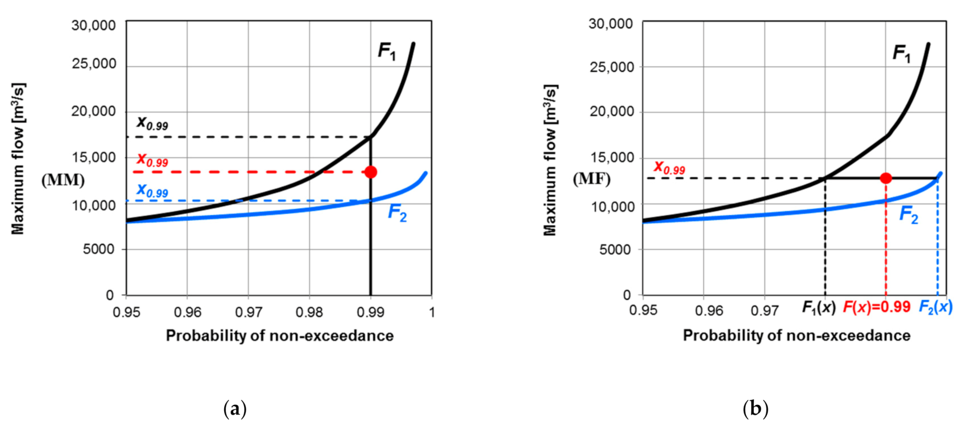
The schematic illustration of two aggregation variants is shown in Figure 3 for two distributions and probability of non-exceedance $p=0.99$. The aggregation procedure can be easily extended to any number of CDFs.

3.3. Aggregation by Quantile Mixture—Mean Magnitude (MM)

Since this variant of aggregation has been presented in detail in our previous papers and also used for non-stationary flood analysis by Debele et al. [39], here only the basic principles of MM aggregation are briefly recalled.

The idea of distributions aggregation assumes that the value of the upper (design) quantile obtained in this way will be less sensitive to the error of the distribution selection, which is a key decision in the analysis of the frequency of floods. The aggregated quantile of the order p $\left({\overline{x}}_p\right)$ is shown schematically in Figure 3a and defined as a weighted average of the form:

$${\overline{x}}_p={\displaystyle \sum }_{i=1}^m{w}_i·{\left({\widehat{x}}_p\right)}_i$$

(1)

where ${\left({\widehat{x}}_p\right)}_i$ is the quantile calculated on the basis of i-th from among m considered distributions, and $w_i$ is the weight assigned to a subsequent distribution. The weights are determined on the basis of the $AI{C}_i$ criterion value as:

$$w_i=\frac{exp\left(-\frac{1}{2}{\delta }_i\right)}{{{\displaystyle \sum }}_{k=1}^{m}exp\left(-\frac{1}{2}{\delta }_k\right)}$$

(2)

where:

$${\delta }_i=AI{C}_i-\min \left(AI{C}_1,\dots ,AI{C}_m\right),i=1,\dots ,m$$

(3)

are the differences between the AIC criterion value for a given model and the smallest value in the whole set, which indicates the best model.

The weights $w_i$ for models with the same number of parameters are expressed by the likelihood function:

$$w_i=\frac{L_i{}^{max}}{{{\displaystyle \sum }}_{k=1}^m{L}_k{}^{max}}$$

(4)

and, like in Equation (2), they can be interpreted as the probability that the data are derived from the i-th of the m distributions considered. If we assume a priori that equally probable candidate distributions $\{M_i,i=1,\dots ,m\}$ with equal number of parameters form a population of distributions M, then the reliability (probability) of the M_i model conditioned by observed flow series $\{x_j,j=1,\dots ,n\} \left(data\right)$ can be specified as:

$$P\left(M_i|data\right)=\frac{P\left(data|M_i\right)}{P\left(data|M\right)}=\frac{P\left(data|M_i\right)}{{{\displaystyle \sum }}_{k=1}^{m}P\left(data|M_k\right)}=\frac{L_i{}^{max}{\left(dx\right)}^n}{{{\displaystyle \sum }}_{k=1}^m{L}_k{}^{max}{\left(dx\right)}^n}=\frac{L_i{}^{max}}{{{\displaystyle \sum }}_{k=1}^m{L}_k{}^{max}}=w_i$$

(5)

This conclusion results directly from the definition of probability and is a special case of the Bayesian model averaging (BMA) [40,41].

3.4. Aggregation by Probability Mixture—Mean Frequency (MF)

To the best of our knowledge, so far there has been no proposal in the literature to aggregate distributions by averaging probabilities of non-exceedance using the weights defined by Equation (5). However, there is literature on probability mixtures models where the weights are assessed by proportion of elements coming from different populations or estimated as additional parameters in estimating procedure, e.g., [42].

Aggregation of candidate distributions according to the probability of non-exceedance, shown schematically in Figure 3b, can be defined by a formula similar to Equation (1) in the MM variant, namely:

$$\overline{F}\left(x_{\overline{p}}\right)={{\displaystyle \sum }}_{i=1}^m{w}_i{\widehat{F}}_i\left(x_{\overline{p}}\right)$$

(6)

where $\overline{F}$ is the cumulative distribution function of the aggregated distribution, ${\widehat{F}}_i$ are distribution functions of the candidates, and the weights $w_i$ are determined on the basis of the AIC value, as in the MM variant. Note that $\overline{F}\left(x_{\overline{p}}\right)=\overline{p}$, but ${\widehat{F}}_i\left(x_{\overline{p}}\right)\ne \overline{p}$ as presented in Figure 3b.

Equation (6) for two distributions takes the form:

$$\overline{F}\left(x_{\overline{p}}\right)=w_1{\widehat{F}}_1\left(x_{\overline{p}}\right)+w_2{\widehat{F}}_2\left(x_{\overline{p}}\right)$$

(7)

Therefore, the density function for the aggregated distribution $\overline{F}$ is determined by Equation (8):

$$f\left(x_{\overline{p}}\right)=w_1{f}_1\left(x_{\overline{p}}\right)+w_2{f}_2\left(x_{\overline{p}}\right)$$

(8)

where $f_1$ and $f_2$ are the probability density functions of the distributions that are averaged. Similar to the averaging of quantiles, the averaging of probabilities is also a special case of the Bayesian model averaging BMA.

4. Accuracy of Aggregated Quantile

4.1. Analytical vs. Numerical Form of Standard Error

The assessment of the accuracy of the design quantile estimates is an essential part of the estimation procedure, which was missing in our previous studies on the MM aggregation method.

To determine the accuracy of quantile estimate, two measures are used: the standard error (SE), which results from the randomness of the sample based on which we make the estimation, and the systematic error (B—bias), which results from the approximation the unknown population distribution by assumed distribution. The general formulas for SE and B errors of quantile estimate ${\widehat{x}}_p$ are given by Equations (9) and (10), respectively:

$$SE\left({\widehat{x}}_p\right)=\sqrt{var\left({\widehat{x}}_p\right)}=\sqrt{E\left[{\widehat{x}}_p-E{\left({\widehat{x}}_p\right)}^2\right]}$$

(9)

$$B\left({\widehat{x}}_p\right)=E\left[{\widehat{x}}_p-x_p\right]$$

(10)

Both types of error are contained in the mean square error (MSE) or in the root of the mean square error (RMSE):

$$RMSE\left({\widehat{x}}_p\right)=\sqrt{S{E}^2\left({\widehat{x}}_p\right)+B^2\left({\widehat{x}}_p\right)}$$

(11)

The value of true quantile is obviously unknown and in hydrological practice of the FFA the bias error is not determined. If the distribution used is accepted by goodness of fit tests, we expect that the bias error of the design quantiles, resulting from the incorrect selection of the statistical model, will be small in comparison with the accuracy of the maximum flow data, for example, and therefore the bias value will be irrelevant. Nevertheless, in the literature, there are papers concerning the simulation studies on the accuracy of the estimates of large quantiles under the assumption of true and then false hypothetical distribution with applying various estimation methods [27,43,44,45]. It has been shown that, in the case of wrong distribution assumption, the MLM method gives the largest bias of the estimates of high quantiles among all estimation methods, and the bias generally increases with increasing sample size.

Nowadays, due to the increasing possibilities of computational techniques and development of statistical software, to calculate the standard error, the Monte Carlo simulation methods, bootstrap techniques are used, or the so-called likelihood function profile method when the MLM estimation method is applied. All these methods are intensive computationally and give, in fact, reliable assessment of quantile estimation error, but their results refer only to the analyzed specific cases. Due to the possibility of comparing the effectiveness of various estimation methods and for the simplicity of calculations, the analytical form of assessing the asymptotic standard error is of greater value. Hence, the analytical formula for the SE of p-order quantile is derived here for both aggregation variants.

4.2. Asymptotic Standard Error of Quantiles from the MM Method

The squared bias of the p-order quantile obtained by the MM aggregation method $\left({\overline{x}}_p\right)$ with respect to a real, unknown value from the population $\left(x_p\right)$ can be expressed by a formula:

$${\left({\overline{x}}_p-x_p\right)}^2={{\displaystyle \sum }}_{i=1}^m{w}_i{\left({\left({\widehat{x}}_p\right)}_i-x_p\right)}^2-{{\displaystyle \sum }}_{i=1}^m{w}_i{\left({\left({\widehat{x}}_p\right)}_i-{\overline{x}}_p\right)}^2$$

(12)

The first term of the expression on the right side of Equation (12) is the square deviation of quantiles estimated by the models included in the analysis, and the second is a measure of the diversity of quantiles of aggregated models. From Equation (12), it follows directly that the greater the diversity of models, the smaller the bias in assessing the aggregate model. Of course, as the variety of models increases, the value of the first component also increases. When choosing models, it is necessary to maintain the right proportions between model diversity and their accuracy [31,33,46].

To derive the analytical formula for the asymptotic standard error of the aggregated quantile from the MM method, let us assume that ${\overline{x}}_p$ is an aggregate quantile based on two candidate distributions 1 and 2, and their quantile estimates of the p-order are ${\left({\widehat{x}}_p\right)}_1$ and ${\left({\widehat{x}}_p\right)}_2$, respectively. According to Equation (1), there is an equality:

$${\overline{x}}_p=w_1·{\left({\widehat{x}}_p\right)}_1+w_2·{\left({\widehat{x}}_p\right)}_2$$

(13)

Since ${\overline{x}}_p$, ${\left({\widehat{x}}_p\right)}_1,$ and ${\left({\widehat{x}}_p\right)}_2$ are random variables, the variance of the quantile $var\left({\overline{x}}_p\right)$ can be determined:

$$\begin{array}{cc}\hfill var({\overline{x}}_p)& =var\left(w_1·{\left({\widehat{x}}_p\right)}_1+w_2·{\left({\widehat{x}}_p\right)}_2\right)\hfill \\ & =w_1^2·var\left({\left({\widehat{x}}_p\right)}_1\right)+w_2^2·var\left({\left({\widehat{x}}_p\right)}_2\right)+2·w_1·w_2·cov\left({\left({\widehat{x}}_p\right)}_1,{\left({\widehat{x}}_p\right)}_2\right)\hfill \\ & =w_1^2·var\left({\left({\widehat{x}}_p\right)}_1\right)+w_2^2·var\left({\left({\widehat{x}}_p\right)}_2\right)+2·w_1·w_2·p\sqrt{var\left({\left({\widehat{x}}_p\right)}_1\right)}\sqrt{var\left({\left({\widehat{x}}_p\right)}_2\right)}\hfill \end{array}$$

(14)

As the quantile estimates ${\left({\widehat{x}}_p\right)}_1$ and ${\left({\widehat{x}}_p\right)}_2$ were calculated based on the same series of data, they are positively, strongly dependent, and the upper limit of the correlation coefficient p is 1. Assuming $p=1$, we obtain:

$$var({\overline{x}}_p)\le {\left(w_1·\sqrt{var\left({\left({\widehat{x}}_p\right)}_1\right)}+w_2·\sqrt{var\left({\left({\widehat{x}}_p\right)}_2\right)}\right)}^2$$

(15)

Thus, the standard error of the aggregate quantile can be estimated as:

$$SE({\overline{x}}_p)\cong w_1·\sqrt{var\left({\left({\widehat{x}}_p\right)}_1\right)}+w_2·\sqrt{var\left({\left({\widehat{x}}_p\right)}_2\right)}$$

(16)

For more candidate distributions $\left(m\right)$, the formula for the asymptotic standard quantile error takes the form:

$$SE({\overline{x}}_p)\cong {\displaystyle \sum }_{i=1}^m{w}_i·\sqrt{var\left({\left({\widehat{x}}_p\right)}_i\right)}$$

(17)

The estimates of p-order quantile variances for individual distributions in Equations (14)–(17) can be determined using the delta method [47,48], or the solutions presented in the literature can be used [7,23,24,25,26,27,28,29,30,31,32,33,34,35,36,37,38,39,40,41,42,43,44,45,46,47,48,49,50].

In addition, it can be proved that the distribution of aggregated quantile is an asymptotically normal distributed with a variance given by Equation (14), like the p-order quantile distribution in individual models. However, the estimates of individual quantiles ${\left({\widehat{x}}_p\right)}_1$, ${\left({\widehat{x}}_p\right)}_2$, and, as a consequence, the estimates of the aggregated quantile ${\overline{x}}_p$ are biased. As mentioned before, the bias results from the fact that the distributions used are models approximating only the unknown distribution of the population. Therefore, various estimation methods, including the MLM method used here, lead to biased quantile estimates, especially in the range of the upper tail of distribution. The bias cannot be determined or removed without knowing the true distribution, and thus remains unknown. Therefore, in the classical flood frequency modeling, a systematic error (bias) is not included because it cannot be. However, in the case of a multi-model approach, we can reduce the bias of the quantiles ${\left({\widehat{x}}_p\right)}_1, {\left({\widehat{x}}_p\right)}_2$ related to the real, unknown value in the population by taking into account their bias in relation to the aggregated quantile, which usually better describes the true quantile value than individual candidate distributions.

Based on Equations (9)–(11), the RMSE of the quantile ${\left({\widehat{x}}_p\right)}_i$ from the i-th model with respect to the aggregated quantile ${\overline{x}}_p$ is expressed by Equation (18):

$$RMSE\left({\left({\widehat{x}}_p\right)}_i\right)=\sqrt{var\left({\left({\widehat{x}}_p\right)}_i\right)+{\left({\left({\widehat{x}}_p\right)}_i-{\overline{x}}_p\right)}^2}$$

(18)

while the $RMSE$ of the aggregated quantile by the MM aggregation for m distributions is equal to:

$$RMSE\left({\overline{x}}_p\right)={\displaystyle \sum }_{i=1}^m{w}_i\sqrt{var\left({\left({\widehat{x}}_p\right)}_i\right)+{\left({\left({\widehat{x}}_p\right)}_i-{\overline{x}}_p\right)}^2}$$

(19)

4.3. Simulation Experiment on the Accuracy of Standard Error Formulas

In order to check how accurate is the approximation of the standard error of the quantile ${\overline{x}}_p$ by Equations (17) and (19), a numerical experiment was carried, which involved:

• generating a 1000-element series of data from a given probability distribution serving as a population distribution
• fitting to the generated sample of two different distributions, determination of their weights, p-order quantiles and aggregated quantile according to Equation (1)
• generating 10,000 N-element data series from the population distribution
• matching to each data series of two selected (in point 2) distributions, determining the weights of both distributions, the values of the aggregated quantile (Equation (1)), its asymptotic standard error (Equations (17) and (19)) and the confidence interval with a confidence level of 68.3%, called a one-sigma confidence interval [39,51].

Generalized exponential distribution (GE) with the mean $\mu$ = 500 and coefficient of variation $Cv=\sigma /\mu$ = 0.5 was used as the population distribution, and gamma (Ga) and log-normal (LN) distributions were assumed as models. In the experiment, the two-parameter distributions were used. The sample length was 50, which corresponds to the average length of the observation series of the seasonal and annual maximum flows in Poland. The assumptions of the experiment, i.e., $Cv$ value and type of model distributions, are consistent with the hydrological regime of many Polish rivers. The results of quantile estimation are shown in

Table 2. Results of quantiles estimation in the simulation experiment (sample of 1000 elements).

Quantile $x_{0.99}$ in the GE Population (m3/s)	1306.43
Quantile $x_{0.99}$ assuming Ga distribution; estimated by MLM (m3/s)	1205.34
Quantile $x_{0.99}$ assuming LN distribution; estimated by MLM (m3/s)	1391.19
Weight $w_1$ of quantile $x_{0.99}$from Ga distribution (−) (Equation (2))	0.232
Weight $w_1$ of quantile $x_{0.99}$from LN distribution (−) (Equation (2))	0.768
Aggregated (Ga and LN) quantile $x_{0.99}$ (m3/s)	1347.98
Correlation coefficient of quantiles $x_{0.99}$from Ga and LN distributions (−)	0.96

.

The relative asymptotic bias of the aggregated quantile relative to the population quantile is 3.18% and is smaller in its absolute value than for quantile estimates from the Ga (−7.74%) and LN (6.49%) distribution separately. The correlation coefficient of quantiles $x_{0.99}$ from Ga and LN distributions confirms the strong positive dependence of the quantiles and correctness of approximation used in Equation (15).

The variance of 0.99 quantile from the LN distribution was estimated based on Rao and Hamed [7]. The procedure given there is in accordance with other literature sources. Meanwhile, in the case of the variance of 0.99 quantile from the Ga distribution, there are discrepancies in the literature, so three methods were used to determine it:

• approximation according to Rao and Hamed [7]
• the method according to Kaczmarek [49]
• the method according to Banasik et al. [23].

Due to the various approximations proposed by the above authors, the variances of quantile $x_{0.99}$ from the Ga distribution differ from each other. As a consequence, we get three different values of the variance of aggregated quantile determined for each of 10,000 generated 50-element samples, which results in different coverage of the true value of the quantile $x_{0.99}$ from the population by the corresponding 68.3% confidence intervals. The probability of covering the true quantile value by the confidence interval for the three versions of the variance assessment of the quantile from Ga distribution is presented in

Table 3. The coverage probability of the true value of the quantile x_0.99 by the 68.3% confidence interval determined on the basis of Equations (17) and (19) for 10,000 samples of 50 elements and for three ways (authors) of the variance assessment of the quantile from Ga distribution.

Author	Probability of Coverage According to Equation (17) (%)	Probability of Coverage According to Equation (19) (%)
1. Rao and Hamed [7]	61.48	67.23
2. Kaczmarek [49]	63.13	68.39
3. Banasik et al. [23]	69.90	73.79

. The results in the second column present the probability of coverage according to Equation (17), i.e., without taking into account the quantiles bias, while the results in the third column presents the probability of coverage according to Equation (19), i.e., with taking into account the quantiles bias.

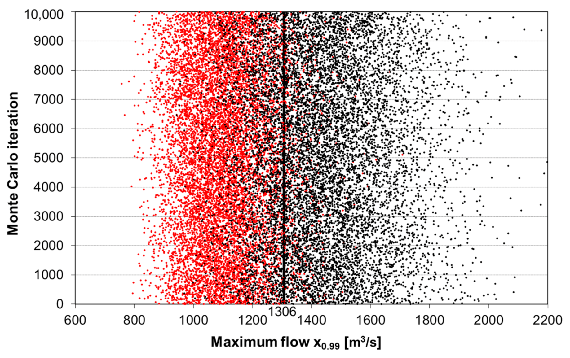
For both Equations (17) and (19), the results for the first two authors of the approximation of the variance of quantile from the Ga distribution are consistent, i.e., for Rao and Hamed [7] and Kaczmarek [49], while the approximation by Banasik et al. [23] yields higher values of the coverage probability than the two previous methods and higher than 68.3%. This suggests that the third method (Banasik et al. [23]) gives an overestimated value of 0.99 quantile variance from the Ga distribution. An illustration of the coverage of the true quantile from population by the confidence intervals according to approximation of Banasik et al. [23] are shown in Figure 4.

Meanwhile, the coverage probability for the first two methods shows that the confidence interval with using the standard error defined by Equation (17) is too narrow (second column in Table 3). The probability of coverage for the first and second methods is approximately 61.5% and 63%, respectively, which is significantly less than 68.3%. A coverage probability of around 68.3% is obtained when, in addition to the standard error, the quantile bias is taken into account according to Equation (19). Thus, the results of the simulation experiment confirm that Equation (17) is an understated approximation of the standard error of quantile in the population.

4.4. Asymptotic Standard Error of Quantile from MF Method

The $x_{\overline{p}}$ quantiles from the $F_1$ and $F_2$ models have asymptotically normal distributions with the variations $va{r}_1\left(x_{\overline{p}}\right)$ and $va{r}_2\left(x_{\overline{p}}\right)$, and are strongly positively dependent. Thus, the variance of the $\overline{p}$-order quantile in the MF distribution is equal to:

$$\begin{array}{cc}\hfill var\left(x_{\overline{p}}\right)& =var\left({\overline{F}}^{-1}\left(\overline{p}\right)\right)=\frac{1}{f^2\left(x_{\overline{p}}\right)}·var\left(\overline{F}\left(x_{\overline{p}}\right)\right)\hfill \\ & =\frac{1}{f^2\left(x_{\overline{p}}\right)}\left(w_1^2·va{r}_1\left({\widehat{F}}_1\left(x_{\overline{p}}\right)\right)+w_2^2·va{r}_2\left({\widehat{F}}_2\left(x_{\overline{p}}\right)\right)+2·w_1·w_2·cov\left({\widehat{F}}_1\left(x_{\overline{p}}\right),{\widehat{F}}_2\left(x_{\overline{p}}\right)\right)\right)\hfill \\ & =\frac{1}{f^2\left(x_{\overline{p}}\right)}\left(w_1^2·f_1^2\left(x_{\overline{p}}\right)·va{r}_1\left(x_{\overline{p}}\right)+w_2^2·f_2^2\left(x_{\overline{p}}\right)·va{r}_2\left(x_{\overline{p}}\right)+2·w_1·w_2·p_{{\widehat{F}}_1\left(x_{\overline{p}}\right),{\widehat{F}}_2\left(x_{\overline{p}}\right)}·\sqrt{va{r}_1\left({\widehat{F}}_1\left(x_{\overline{p}}\right)\right)}·\sqrt{va{r}_2\left({\widehat{F}}_2\left(x_{\overline{p}}\right)\right)}\right)\hfill \\ & =\frac{1}{f^2\left(x_{\overline{p}}\right)}\left(w_1^2·f_1^2\left(x_{\overline{p}}\right)·va{r}_1\left(x_{\overline{p}}\right)+w_2^2·f_2^2\left(x_{\overline{p}}\right)·va{r}_2\left(x_{\overline{p}}\right)+2·w_1·w_2·p_{{\widehat{F}}_1\left(x_{\overline{p}}\right),{\widehat{F}}_2\left(x_{\overline{p}}\right)}·f_1\left(x_{\overline{p}}\right)·f_2\left(x_{\overline{p}}\right)\sqrt{va{r}_1\left(x_{\overline{p}}\right)}·\sqrt{va{r}_2\left(x_{\overline{p}}\right)}\right)\hfill \end{array}$$

(20)

where $p_{{\widehat{F}}_1\left(x_{\overline{p}}\right),{\widehat{F}}_2\left(x_{\overline{p}}\right)}$ is the correlation coefficient between the probabilities of non-exceedance in the ${\widehat{F}}_1$ and ${\widehat{F}}_2$distributions corresponding to the value of $x_{\overline{p}}$. Assuming $p_{{\widehat{F}}_1\left(x_{\overline{p}}\right),{\widehat{F}}_2\left(x_{\overline{p}}\right)}=1$, we obtain a convenient analytical estimate of the upper limit of the quantile variance in MF aggregation, in the form:

$$var\left(x_{\overline{p}}\right)\le {\left(\frac{w_1·f_1\left(x_{\overline{p}}\right)}{f\left(x_{\overline{p}}\right)}·\sqrt{va{r}_1\left(x_{\overline{p}}\right)}+\frac{w_2·f_2\left(x_{\overline{p}}\right)}{f\left(x_{\overline{p}}\right)}·\sqrt{va{r}_2\left(x_{\overline{p}}\right)}\right)}^2$$

(21)

The asymptotic standard error of the estimate of aggregated quantile using the MF method for two distributions is therefore:

$$SE(x_{\overline{p}})\cong \frac{w_1·f_1\left(x_{\overline{p}}\right)}{f\left(x_{\overline{p}}\right)}·\sqrt{va{r}_1\left(x_{\overline{p}}\right)}+\frac{w_2·f_2\left(x_{\overline{p}}\right)}{f\left(x_{\overline{p}}\right)}·\sqrt{va{r}_2\left(x_{\overline{p}}\right)}$$

(22)

and for $m$ distributions, respectively:

$$SE(x_{\overline{p}})\cong {{\displaystyle \sum }}_{i=1}^m\frac{w_i·f_i\left(x_{\overline{p}}\right)}{f\left(x_{\overline{p}}\right)}·\sqrt{va{r}_i\left(x_{\overline{p}}\right)}$$

(23)

The distribution of quantiles corresponding to $x_{\overline{p}}$ in the MF aggregation is asymptotically normal with the approximate variance given by Equation (23) and with the biased mean value. Taking into account the bias of the quantiles of candidate distributions ${\left(x_{\overline{p}}\right)}_i$ in relation to their aggregated value $x_{\overline{p}}$ and assuming the correlation coefficient value between the quantiles equals to 1, we get the assessment of the $RMSE$ of the quantile $x_{\overline{p}}$ in the form:

$$RMSE\left(x_{\overline{p}}\right)\cong {{\displaystyle \sum }}_{i=1}^m\frac{w_i·f_i\left(x_{\overline{p}}\right)}{f\left(x_{\overline{p}}\right)}·\sqrt{va{r}_i\left(x_{\overline{p}}\right)+{\left({\left(x_{\overline{p}}\right)}_i-x_{\overline{p}}\right)}^2}$$

(24)

5. Case Study of MM and MF Methods of Distribution Aggregation

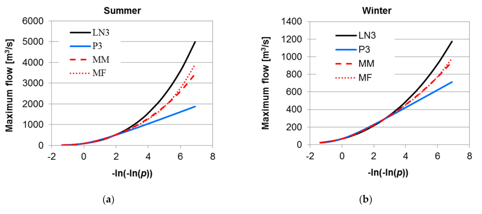
Both methods of aggregation statistical models are used to analyze the synthetic series of the seasonal maximum flows. In each season, two probability distributions are considered: Pearson type 3 distribution (P3) and three-parameter log-normal distribution (LN3), which are aggregated by MM and MF methods. These distributions are illustrated in Figure 5. The weights of the LN3 and P3 distributions are adopted for winter: 0.499 and 0.501, for summer: 0.503 and 0.497. Thus, both distributions describe a series of maximum seasonal flows in a comparatively right way in terms of MLM estimation. If the classical methodology for choosing a better distribution was used, it would be P3 for winter and LN3 for summer.

In Figure 5, instead of the usual probability scale, a reduced Gumbel variable is used to make the differences in distribution tails more visible.

Comparing the MM and MF methods of distribution aggregation with respect to the quantile values, both methods give similar results. The relative differences of the quantiles obtained from the MF and MM methods with respect to the quantile value from MM are presented in Figure 6.

In the range of the probabilities of non-exceedance from ~0.1 to ~0.9, the consistency of the results of both aggregation methods is high. The largest relative differences occur in the upper tail of the probability distribution and increase as the quantile order increases, reaching a value of about 4% for the winter season and about 14% for the summer season. The presented result depends on the selected candidate distributions; however, it should be expected that the general shape of the relationship presented in Figure 6 is similar also for other pairs of distributions.

The results of 0.99 quantile estimation assuming P3 and LN3 distributions, then using MM and MF aggregation, are presented in

Table 4. Comparison of seasonal quantiles x_0.99 and their accuracy expressed by asymptotic errors obtained from various ways of estimation. The superscripts of aggregation methods MM and MF indicate the equation number which was used for the calculations (for two distributions, i.e., m = 2).

	Quantile x0.99 (m3/s)				Accuracy of Quantile x0.99 (m3/s)
					SE (x0.99)				RMSE (x0.99)
Estimation method	LN3	P3	MM	MF	LN3	P3	MM(17)	MF(23)	MM(19)	MF(24)
Summer	2050	1220	1630	1600	565.9	193.7	380.9	379.5	581.4	547.0
Winter	599	482	541	534	124.5	66.3	95.4	92.9	112.8	108.1

along with the quantile uncertainty expressed by the asymptotic standard error (6th–9th columns) and by the root mean square error (10th–11th columns). Thus, the results in the latter two columns include the bias of quantile estimates of LN3 and P3 distributions with respect to the aggregated quantile. For clarity, in the superscript of aggregation methods, we provide the equation number on the basis of which the calculation was made. The Kaczmarek [49] method was applied to assess the variance of the P3 distribution quantile.

One can see a high similarity of 0.99 quantile estimates aggregated by the MM and MF methods, as well as similar compatibility of their SE and RMSE errors, which are slightly smaller for the MF than for MM. The slight difference in the weights assigned to the analyzed distributions makes it possible to change the best matching distribution as the observation series lengthens, and therefore the value of the design quantile can be changed. Meanwhile, the aggregated distributions remain more resistant to such changes.

Similarly, a consistent result is obtained in a numerical experiment. For the 1000 element series, the value of 0.99 quantile aggregated by the MM method is 1347.98 m³/s, while, by the MF method, is 1347.81 m³/s. The difference of two estimates is negligible. When written in the format used by the Polish Hydrological Service, i.e., with three significant digits, both estimate values are equal to 1350 m³/s.

6. Conclusions

An aggregation by a mixture of probabilities of non-exceedance has been proposed in this paper as a new variant of multi-model approach in flood frequency analysis. This method, named mean frequency (MF), is compared with an aggregation by a mixture of quantiles presented in previous authors’ papers and called mean magnitude here (MM). For both aggregation variants, analytical formulas were derived for the asymptotic standard error of the estimate of p-order quantile and for its root mean square error, which takes into account the bias of the estimates of quantiles from the candidate distributions with respect to the aggregated quantile. In the numerical experiment, the correctness of the derived formulas in the MM aggregation was verified, comparing the theoretical and simulated probability of covering the true population quantile by the asymptotic confidence interval (confidence level 68.3%).

The MM aggregation can be interpreted as measuring the same quantity with various measuring instruments whose role is played by the candidate distributions. Averaging the results of such “measurements” corresponds to the idea of reducing measurement uncertainty by averaging the results of various measurements. The MF approach is based on the assumption that the measurement series is subject to a probability distribution, which is a mixture of candidate distributions in the proportions determined by the assigned weights w_i.

Due to the possibility of wide use of MM and MF aggregation methods in various (broad) calculations, e.g., quantiles of the distribution of annual peak flows, the following issues should be noted:

When using the MM and MF aggregation methods in practice, the following issues should be noted:

• the MM method allows for determining the p-order quantile of aggregated distribution as a simple and explicit form (Equation (1)), while the MF method requires a numerical solution of Equation (6), assuming $\overline{F}\left(x\right)=p$.
• in the MF method, there is an explicit form of the cumulative distribution function and the density function of aggregated distribution $\overline{F}$. In the MM method, these functions can be determined only numerically.
• Calculation of the accuracy of the p-order quantile in the MM method requires the determination of the variance of the same-order quantile for the candidate distributions, in the MF method, it is necessary to determine the variance of quantiles at a wider range of probability values.

Both the current and previous research of the authors on aggregation methods show that these methods prove to be a useful and productive approach to flood frequency analysis. Compared with the classic selection of the best-fit distribution, aggregation methods are less sensitive to wrong model selection and give estimates of design quantiles more stable when extending the observation series. The studies conducted in this article on the two proposed methods of aggregation MM and MF show that:

• Aggregation by quantile mixture (MM) leads to slightly different results than aggregation by probability mixture (MF) with respect both to the p-order quantile value and its uncertainty.
• The largest difference in quantile values from both approaches occurs for high probabilities of non-exceedance as $p>0.99$, i.e., in the upper tail of model distributions.
• In the probability range representing the main mass of the distribution, when the density functions are similar, both aggregation methods are approximately consistent.
• The derived analytical formulas for the asymptotic standard error for MM and MF aggregation can be used to approximate assessment of the accuracy of the p-order quantile, effectively competing with other simulation techniques of this assessment
• A more accurate estimate of the 0.99 quantile accuracy is obtained when the bias of quantiles of candidate distributions is included.
• Taking into account the bias of the quantile from individual distribution F_i in relation to the aggregated quantile allows for reducing the bias of the quantile from distribution F_i relative to the unknown quantile value in the population.

Both quantile and probability mixture models provide a promising tool for parameter estimation that may be useful in various (broad) areas, especially in the life sciences—for example, when some parameters of the experiment are out of the control or when the experiment cannot be repeated under the same conditions. Our research on this subject will be continued.

References

- Blöschl, G.; Hall, J.; Parajka, J.; Perdigão, R.A.P.; Merz, B.; Arheimer, B.; Aronica, G.T.; Bilibashi, A.; Bonacci, O.; Borga, M.; et al. Changing climate shifts timing of European floods. Science 2017, 357, 588–590. [Google Scholar] [CrossRef] [PubMed] [Green Version]
- Blöschl, G.; Hall, J.; Viglione, A.; Perdigão, R.A.P.; Parajka, J.; Merz, B.; Lun, D.; Arheimer, B.; Aronica, G.T.; Bilibashi, A.; et al. Changing climate both increases and decreases European river floods. Nat. Cell Biol. 2019, 573, 108–111. [Google Scholar] [CrossRef] [PubMed]
- Didovets, I.; Krysanova, V.; Bürger, G.; Snizhko, S.; Balabukh, V.; Bronstert, A. Climate change impact on regional floods in the Carpathian region. J. Hydrol. Reg. Stud. 2019, 22, 100590. [Google Scholar] [CrossRef]
- Kundzewicz, Z.W. Changes in Flood Risk in Europe; CRC Press: London, UK, 2019. [Google Scholar]
- Jamshed, A.; Birkmann, J.; McMillan, J.M.; Rana, I.A.; Lauer, H. The Impact of Extreme Floods on Rural Communities: Evidence from Pakistan. In Climate Change, Hazards and Adaptation Options; Leal Filho, W., Nagy, G., Borga, M., Chávez Muñoz, P., Magnuszewski, A., Eds.; Springer: Cham, Switzerland, 2020; pp. 585–613. [Google Scholar] [CrossRef]
- Cunnane, C. Operational Hydrology Report No.33: Statistical Distributions for Flood Frequency Analysis; World Meteorological Organization: Geneva, Switzerland, 1989; ISBN 9789263107183. [Google Scholar]
- Rao, A.R.; Hamed, K.H. Flood Frequency Analysis; CRC Press: Boca Raton, FL, USA, 2000; ISBN 9780849300837. [Google Scholar]
- Strupczewski, W.; Kochanek, K.; Bogdanowicz, E.; Markiewicz, I. On seasonal approach to flood frequency modelling. Part I: Two-component distribution revisited. Hydrol. Process. 2011, 26, 705–716. [Google Scholar] [CrossRef]
- Kochanek, K.; Strupczewski, W.G.; Bogdanowicz, E. On seasonal approach to flood frequency modelling. Part II: Flood frequency analysis of Polish rivers. Hydrol. Process. 2011, 26, 717–730. [Google Scholar] [CrossRef]
- Strupczewski, W.; Kochanek, K.; Feluch, W.; Bogdanowicz, E.; Singh, V.P. On seasonal approach to nonstationary flood frequency analysis. Phys. Chem. Earth Parts A/B/C 2009, 34, 612–618. [Google Scholar] [CrossRef]
- Petrow, T.; Merz, B. Trends in flood magnitude, frequency and seasonality in Germany in the period 1951–2002. J. Hydrol. 2009, 371, 129–141. [Google Scholar] [CrossRef] [Green Version]
- Ozga-Zielinska, M.; Brzezinski, J.; Ozga-Zielinski, B. Guidelines for Flood Frequency Analysis; Long Measurement Series of River Discharge WMO HOMS Component I81.3.01; Institute of Meteorology and Water Management: Warsaw, Poland, 2005. [Google Scholar]
- Ozga-Zielińska, M.; Brzeziński, J.; Ozga-Zieliński, B. Zasady Obliczania Największych Przepływów Rocznych o Określonym Prawdopodobieństwie Przewyższenia przy Projektowaniu Obiektów Budownictwa Hydrotechnicznego. Długie Ciągi Pomiarowe Przepływów. [Guidelines for the Determining the Annual Maximum Flows with a Certain Probability of Exceedance in the Design of Hydrotechnical Structures. Long Data Series of Flows]; Materiały Badawcze, Seria: Hydrologia i Oceanologia, 27; IMGW: Warszawa, Poland, 1999. (In Polish) [Google Scholar]
- Strupczewski, W. Częstość wielkich wód. Prz. Geof. X (XVIII) 1965, 1, 83–93. (In Polish) [Google Scholar]
- Debele, S.E.; Bogdanowicz, E.; Strupczewski, W. The impact of seasonal flood peak dependence on annual maxima design quantiles. Hydrol. Sci. J. 2017, 62, 1603–1617. [Google Scholar] [CrossRef] [Green Version]
- Salvadori, G.; De Michele, C. Frequency analysis via copulas: Theoretical aspects and applications to hydrological events. Water Resour. Res. 2004, 40, 1–17. [Google Scholar] [CrossRef]
- Durrans, S.R.; Eiffe, M.A.; Thomas, W.O.; Goranflo, H.M. Joint Seasonal/Annual Flood Frequency Analysis. J. Hydrol. Eng. 2003, 8, 181–189. [Google Scholar] [CrossRef]
- Ye, W.; Wang, C.; Xu, X. On seasonal and semi-annual approach for flood frequency analysis. Stoch. Environ. Res. Risk Assess. 2017, 32, 51–62. [Google Scholar] [CrossRef]
- U.S. Water Resources Council. Guidelines for Determining Flood Flow Frequency Bull 17B Hydrol. Comm.; U.S. Water Resources Council: Washington, DC, USA, 1982.
- FEH. Flood Estimation Handbook 3: Statistical Procedures for Flood Frequency Estimation; Institute of Hydrology: Wallingford, UK, 1999; ISBN 9781906698003. [Google Scholar]
- Griffis, V.W.; Stedinger, J.R. Evolution of Flood Frequency Analysis with Bulletin 17. J. Hydrol. Eng. 2007, 12, 283–297. [Google Scholar] [CrossRef]
- Zasady Obliczania Największych Przepływów Rocznych o Określonym Prawdopodobieństwie Pojawiania się Przy Projektowaniu Urządzeń Inżynierskich i Urządzeń Hydrotechnicznych Gospodarki Wodnej w Zakresie Budownictwa Hydrotechnicznego; Central Office of Water Management: Warsaw, Poland, 1969. (In Polish)
- Banasik, K.; Wałęga, A.; Węglarczyk, S.; Więzik, B. Aktualizacja Metodyki Obliczania Przepływów i Opadów Maksymalnych o Określonym Prawdopodobieństwie Przewyższenia dla Zlewni Kontrolowanych i Niekontrolowanych Oraz Identyfikacji Modeli Transformacji Opadu w Odpływ [Updating of the Methodology for Determining Maximum Flows and Rainfall of a Set Probability of Exceedance for Controlled and Uncontrolled Catchments and Identification of Models of Transformation of Precipitation into Outflow]; National Water Management Board, Association of Polish Hydrologists: Warsaw, Poland, 2017. (In Polish)
- Stedinger, J.R.; Vogel, R.M.; Foufoula-Georgiou, E. Frequency analysis of extreme events. In Handbook of Hydrology; Maidment, D.R., Ed.; McGraw Hill: New York, NY, USA, 1993; Chapter 18. [Google Scholar]
- Bobée, B.; Rasmussen, P.F. Recent advances in flood frequency analysis. Rev. Geophys. 1995, 33, 1111–1116. [Google Scholar] [CrossRef]
- Rizwan, M.; Guo, S.; Xiong, F.; Yin, J. Evaluation of Various Probability Distributions for Deriving Design Flood Featuring Right-Tail Events in Pakistan. Water 2018, 10, 1603. [Google Scholar] [CrossRef] [Green Version]
- Strupczewski, W.; Mitosek, H.T.; Kochanek, K.; Singh, V.P.; Weglarczyk, S. Probability of correct selection from lognormal and convective diffusion models based on the likelihood ratio. Stoch. Environ. Res. Risk Assess. 2006, 20, 152–163. [Google Scholar] [CrossRef]
- Mitosek, H.; Strupczewski, W.; Singh, V.P. Three procedures for selection of annual flood peak distribution. J. Hydrol. 2006, 323, 57–73. [Google Scholar] [CrossRef]
- Ouarda, T.B.M.J.; Ashkar, F.; Bensaid, E.; Hourani, I. Statistical Distributions Used in Hydrology. Transformations and Asymptotic Properties; Scientific Report; Department of Mathematics, University of Moncton: Moncton, NB, Canada, 1994; p. 31. [Google Scholar]
- El Adlouni, S.; Ouarda, T.B.M.J.; Bobée, B. Orthogonal projection L-moment estimators for three-parameter distributions. Adv. Appl. Stat. 2007, 7, 19–209. [Google Scholar]
- Bogdanowicz, E. Podejście wielomodelowe w zagadnieniach estymacji kwantyli rozkładu wartości maksymalnych [Multimodel approach to estimation of extreme value distribution quantiles]. In Monografie Komitetu Inżynierii Środowiska Polskiej Akademii Nauk; Więzik, B., Ed.; Wydawnictwa KGW PAN: Warsaw, Poland, 2010; Volume 68, pp. 57–70. ISBN 9788389293930. (In Polish) [Google Scholar]
- Markiewicz, I.; Strupczewski, W.G.; Bogdanowicz, E.; Kochanek, K. Generalized Exponential Distribution in Flood Frequency Analysis for Polish Rivers. PLoS ONE 2015, 10, e0143965. [Google Scholar] [CrossRef]
- Markiewicz, I.; Bogdanowicz, E.; Kochanek, K. On the Uncertainty and Changeability of the Estimates of Seasonal Maximum Flows. Water 2020, 12, 704. [Google Scholar] [CrossRef] [Green Version]
- Kendall, M.G.; Stuart, A. The advanced theory of statistics; Vol. 2. Inference and Relationship; Charles Griffin and Company Limited: London, UK, 1973. [Google Scholar]
- Kaczmarek, Z. Statistical Methods in Hydrology and Meteorology; Published for the Geological Survey; US Department of the Interior and the National Science Foundation: Washington, DC, USA; Foreign Scientific Publications Department of the National Centre for Scientific, Technical and Economic Information: Warsaw, Poland, 1977.
- Akaike, H. A new look at the statistical model identification. IEEE Trans. Autom. Control. 1974, 19, 716–723. [Google Scholar] [CrossRef]
- Wolfram, S. The Mathematica Book, 4th ed.; Wolfram Media, Cambridge University Press: Cambridge, UK, 1999; ISBN 0521643147. [Google Scholar]
- Strupczewski, W.G.; Kochanek, K.; Markiewicz, I.; Bogdanowicz, E.; Weglarczyk, S.; Singh, V.P. On the tails of distributions of annual peak flow. Hydrol. Res. 2011, 42, 171–192. [Google Scholar] [CrossRef] [Green Version]
- Debele, S.E.; Strupczewski, W.G.; Bogdanowicz, E. A comparison of three approaches to non-stationary flood frequency analysis. Acta Geophys. 2017, 65, 863–883. [Google Scholar] [CrossRef]
- Volinsky, C.T.; Raftery, A.E.; Madigan, D.; Hoeting, J.A. David Draper and E. I. George, and a rejoinder by the authors. Stat. Sci. 1999, 14, 382–417. [Google Scholar] [CrossRef]
- Laio, F.; Di Baldassarre, G.; Montanari, A. Model selection techniques for the frequency analysis of hydrological extremes. Water Resour. Res. 2009, 45. [Google Scholar] [CrossRef]
- Szulczewski, W.; Jakubowski, W. The Application of Mixture Distribution for the Estimation of Extreme Floods in Controlled Catchment Basins. Water Resour. Manag. 2018, 32, 3519–3534. [Google Scholar] [CrossRef] [Green Version]
- Strupczewski, W.G.; Singh, V.P.; Weglarczyk, S. Asymptotic bias of estimation methods caused by the assumption of false probability distribution. J. Hydrol. 2002, 258, 122–148. [Google Scholar] [CrossRef]
- Weglarczyk, S.; Strupczewski, W.G.; Singh, V.P. A note on the applicability of log-Gumbel and log-logistic probability distributions in hydrological analyses: II. Assumed pdf. Hydrol. Sci. J. 2002, 47, 123–137. [Google Scholar] [CrossRef] [Green Version]
- Markiewicz, I.; Strupczewski, W.G.; Kochanek, K. On accuracy of upper quantiles estimation. Hydrol. Earth Syst. Sci. 2010, 14, 2167–2175. [Google Scholar] [CrossRef] [Green Version]
- Gatnar, E. Podejście Wielomodelowe w Zagadnieniach Dyskryminacji i Regresji [A Multi-Model Approach to Issues of Discrimination and Regression]; Wydawnictwa Naukowe PWN: Warsaw, Poland, 2008. (In Polish) [Google Scholar]
- Dorfman, R. A note on the delta-method for finding variance formulae. Biom. Bull. 1938, 1, 129–137. [Google Scholar]
- Oehlert, G.W. A Note on the Delta Method. Am. Stat. 1992, 46, 27–29. [Google Scholar] [CrossRef]
- Kaczmarek, Z. Przedział ufności jako miara dokładności oszacowania przepływów powodziowych [Confidence interval as a measure of accuracy of estimation of flood flows]. Wiadomości Służby Hydrol. Meteorol. 1960, 7, 133–185. (In Polish) [Google Scholar]
- Kite, G.W. Frequency and Risk Analysis in Hydrology; Water Resources Publications: Fort Collins, CO, USA, 1977. [Google Scholar]
- Woodall, W.H.; Wheeler, D.J.; Chambers, D.S. Understanding Statistical Process Control. Technometrics 1986, 28, 402. [Google Scholar] [CrossRef]
Publisher’s Note: MDPI stays neutral with regard to jurisdictional claims in published maps and institutional affiliations. |
Figure 1.
Data of the Koszyce Wielkie gauging station on the Biała Tarnowska river: (a) location in Poland; (b) observed summer maximum flows.
Figure 2.
The quantiles x0.99 of the best (according to the AIC criterion) distribution of the maximum summer flows in Koszyce Wielkie station along with an increasing number of observation series and quantiles aggregated by quantile magnitude method (MM) from candidate distributions. Key to the distributions: Ga—Gamma, We—Weibull, GE—Generalized exponential, IG—Inverse Gaussian, LN—Log-normal.
Figure 3.
Two schemes of aggregating distributions: (a) aggregation of quantiles (MM—mean magnitude); (b) aggregation of probabilities of non-exceedance (MF—mean frequency).
Figure 4.
Realization of 68.3% confidence intervals against the true quantile value in the population. Red dots correspond to the beginnings and black to the ends of the intervals.
Figure 5.
The cumulative distribution functions of maximum seasonal flows along with aggregated models using MM and MF methods: (a) in summer; (b) in winter.
Figure 6.
The difference between quantiles of the same order in MF and MM approach expressed in (%) of MM value: (a) aggregated summer quantile; (b) aggregated winter quantile.