Decadal Spatiotemporal Halocline Analysis by ISAS15 Due to Influx of Major Rivers in Oceans and Discrepancies Illustrated Near the Bay of Bengal

Abstract

The discharge from rivers is one of the major factors of regional salinity perturbations in addition to precipitation, evaporation, and circulation of the ocean, whereas simulations regarding the marine environment are dominantly affected by ocean salinity. Moreover, perturbations in the timing and quantity of freshwater cause salinity fluctuations, which in turn, affect the communities of both plant and fauna. In this regard, the study ingeniously employs In Situ Analysis System-15 (ISAS15) data, which is freely available online, to ascertain the salinities in proximity of the major rivers around the globe. Such computations are multilayered, i.e., for 1, 3, 5, and 10 m, and conducted along major freshwater influxes, i.e., the Amazon River, Bay of Bengal (BoB), and Yangtze River, on decadal scales, i.e., in 2004 and in 2014. Depending upon the location and availability of ISAS-15 data, the area in proximity of the Amazon is analyzed horizontally, vertically, and obliquely, whereas the areas in proximity of the BoB and Yangtze estuary are analyzed vertically and obliquely. Similarly, the study analyzed the freshwater influx at the aforementioned locations both for the maxima and minima, i.e., during the particular months that observed the maximum and minimum influx into the ocean from the above-mentioned freshwater sources in 2004, as well as in 2014. The detailed analysis proved the outcomes to be conforming with the documented literary data along the Amazon and Yangtze estuaries. However, the computed analysis illustrated the anomalous values in proximity of the BoB. The study proceeds to discuss an ingenious approach of computing, as well as extrapolating, the salinities, temperatures, and sound speed profiles (SSPs) by employing in situ deep Argo data in order to counter such anomalies, as well as conjoin it with ISAS data, to investigate such regions with broader spatiotemporal capabilities for the future course of action. For this particular study, this method is employed on certain Argo buoys in order to prove the efficacy of the aforementioned novel approach.

1. Introduction

The estuary’s salinity perturbation is responsible for a distinctive and elementary role in constructing spatial patterns of biota, physical characteristics, and certain biogeochemical procedures. Such salinity variations are caused by the influx of freshwater into the sea among other reasons such as precipitation, evaporation, and circulation of the ocean. These perturbations not only lower the salinity in the near-surface layer but can also create habitat instability for communities of both animal and fauna. Furthermore, the average sea level has gone through an intense hike during the entire previous century on a global scale. The reason behind such a hike can be ascribed to both ocean warming and rising continental freshwater influx [1,2,3,4,5]. In order to ascertain temporal weather fluctuations relying on seasonal to decadal perturbations, an array of 3000 floats offering vertical profiles of CTD (Conductivity, Temperature, and Depth) in global oceans to the depths of 2000 m in almost real-time was proposed by the end of the previous century and was named the Argo Array. The connectivity of this array with other networks was proposed in order to offer a weather observing model on a global scale. This array was also meant to provide the data required to calibrate the satellite data [6,7,8]. This array offered coverage on the basis of 3° latitude × 3° longitude × 10-day cycles. In 2015, another array of 1228 floats was proposed (which is already in the process of deployment) to cover the deeper half of the ocean and was named the Deep Argo array, and it will offer global coverage on the basis of 5° latitude × 5° longitude × 15 day cycles upon its global deployment. These arrays, along with the method proposed in this study at the end of the results, cover for the poor observational coverage, as well as insufficient perspective of the interchange of the entire components of the water cycle [4,9]. Moreover, an interpolation tool that performs optimally is evolved to generate worldwide monthly regions of both salinities and temperatures from Argo data combined with monitoring from varying networks on a 0.5° grid, and having a vertical resolution of 152 levels initiating from 0 to 2000 m depth and covariances defined for every grid point. This tool is termed the In-Situ Analysis System (ISAS) and is capable of maintaining the temporal and spatial sampling abilities of the aforementioned Argo array. This ISAS has been improved since the performance of initial global re-analysis in 2009 by comprising all kinds of vertically accumulated profiles in addition to time series. The gridded regions for the ISAS are thoroughly dependent on in-situ measurements. The tool being employed in this particular study is In Situ Analysis System-15 (ISAS15), which covers the temporal duration of 2002 to 2015, and certain regions in the form of horizontal, vertical, or oblique lines are selected in proximity of the Amazon, Bay of Bengal (BoB), and Yangtze estuaries, as depicted in Tables 1–3 in the ensuing section, respectively. As this tool only employs delayed mode in situ data, it comprises the best-quality products in Delayed Mode. In addition, pre-processing is performed on data, and extra-QC (Quality Control) devoted to the ISAS15 analyses is conducted on in situ profiles prior to their inclusion in the analysis [10,11,12,13]. Despite inclusion of such carefully analyzed data, this study found some discrepancies in proximity of the BoB while analyzing the halocline on the decadal scale for both minima and maxima months, which may rely on multiple factors. The study offers an ingenious method that involves the aforementioned core Argo, Deep Argo, and the extrapolations based on these floats to ascertain and verify the salinities, temperatures, and sound speed profiles (SSPs) at such locations. In addition, the study analyzed the halocline in proximity of the Amazon’s (Brazil) freshwater influx area, along with the Yangtze River (China). The measures at these two locations are in accordance with the documented literature and offered the salinity perturbations according to the freshwater influx for both maxima and minima months. The time-related pattern of freshwater influx varies hugely among varying rivers, i.e., their locality within an annual cycle varies on the riverine-estuarine spectrum. The Amazon river is a major source of discharge into the Atlantic Ocean amounting to nearly 17%, i.e., $6300 \times {10}^9 {\mathrm{m}}^3{\mathrm{year}}^{-1}$, of the worldwide riverine influx to the oceans. The maxima influx for this river occurs in May and June, which is three times greater than that during the minima duration, which is December to January. The research has indicated its effects on sea level, as well as on salinity and temperature perturbations, to be of higher consideration for both regional and global scales. The research activity around the Amazon River starts 70.2 km away from the shore at the location of 49.46 W and 0.06 N. The vertical computations of salinity are toward 833.91 km from this particular position, 834.337 km of horizontal computations, and 1177.33 km of computations along the oblique distance [14,15,16,17]. Similarly, the BoB is quite huge with a length of 2090 km and width of 1610 km as it borders with India and Sri Lanka on the western side, with Bangladesh on the northern side and Myanmar and Thailand on the eastern side. However, our major concern is to monitor this bay initiating from the side near Bangladesh to the south roughly 750 km both vertically and obliquely, as will be detailed in the ensuing section. The BoB is considered among the highest freshwater influxes around the global oceans with an annual discharge of $970 \times {10}^9 {\mathrm{m}}^3{\mathrm{year}}^{-1}$ from Ganges-Brahmaputra and $430\times {10}^9{\mathrm{m}}^3{\mathrm{year}}^{-1}$ from Irrawaddy (Burma) as the major sources of influx in the BoB. The freshwater influx causes the salinity to drop by roughly 7 psu, especially in the far northern region. This low-saline water flows southward near the Indian coast as the reversal of the East India Coastal Current from August to December. The study region for this particular activity starts 82.19 km away from the shore at a location of 91 E, 22.24 N. It is computed 794.12 km for the vertical dimension and 1122.87 km obliquely [14,18,19]. Finally, the Yangtze River is considered the longest river, i.e., 6300 km, ranking fifth largest in terms of freshwater influx of $900 \times {10}^{9 }{\mathrm{m}}^3{\mathrm{year}}^{-1}$ annually and the biggest estuary within China comprising three bifurcations and four channels into the sea. The starting position for this particular activity around the Yangtze initiates 105.16 km away from the coast at a location of 121.9 E, 31.3 N [14,20,21]. The study offers an ingenious method ascertaining the halocline perturbations both spatially and temporally from an online dataset, i.e., ISAS-15, which is free of charge. In addition, the study offers yet another ingenious method based on the least squares method, which conjoins core (covering 3° latitude × 3° longitude × 10-day cycles) and deep Argo (covering 5° latitude × 5° longitude × 15 day cycles) float’s data in order to extrapolate to abyssal oceans to offer wider spatiotemporal coverage, as well as to verify any anomalous, ambiguous, or erroneous outcomes [22]. The further details regarding the experimental setup and precise locations with time are illustrated in the ensuing section.

2. Methods

As mentioned earlier, the ISAS15 datasets are employed for this particular study, which analyzes the halocline at three locations, i.e., Amazon river influx in the Atlantic Ocean, the BoB near Bangladesh’s rivers influx, Yangtze River’s influx in the East China Sea. The results are presented in terms of salinity units, i.e., in psu, along the distance of vertical, horizontal, or oblique in kilometers (km) accordingly depending on the availability of ISAS-15 data. Furthermore, the results are presented in multilayers, i.e., at 1, 3, 5, and 10 m. The results are illustrated both in 2D scales. Finally, the results are exhibited both for the maxima, i.e., maximum freshwater influx month, as well as for the minima, i.e., minimum freshwater influx during both 2004 and 2014, in order to offer the decadal halocline analysis accordingly. These maxima and minima months are then compared with each other for the varying years, i.e., for 2004 and 2014. The outcomes along the Amazon and Yangtze river are as expected, whereas apparent discrepancies are observed in the BoB. An ingenious and novel approach mentioned in the previous section is described at the end of the results section, which hints at rectifying such discrepancies innovatively. The detailed methodology along each river’s influx is explained in the ensuing subsections.

2.1. Analysis along the Amazon River

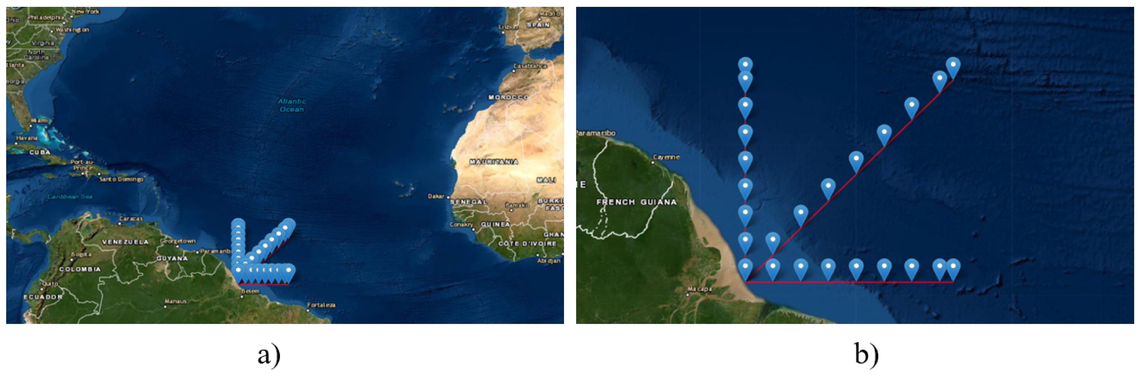
The area chosen for the analysis is 70.2 km away from the delta at a location of 49.46 W, 0.06 N as mentioned earlier. This particular region is measured in three dimensions, i.e., vertically, horizontally, and obliquely. The vertical computations initiated from the starting location of 49 W, 0.499994 N to 49 W, 7.974132 N, covering a distance of 833.91 km. The horizontal computations initiated from 49 W, 0.499994 N to 41.5 W, 0.499994 N, covering a distance of 834.33 km. Finally, the oblique computations initiated from 49 W, 0.499994 N to 41.5 W, 7.974132 N, covering a distance of 1177.33 km. These particular distances along the vertical, horizontal, and oblique lines are illustrated both globally and focused in Figure 1a,b, respectively. Similarly, the exact coordinates in latitude and longitude are depicted, where Lat And Long are abbreviated for latitude and longitude, respectively, and V, H, and O represent vertical, horizontal, and oblique, respectively, as depicted in

Table 1. This table presents details of the computed coordinates along the Amazon Estuary.

Serial No.	Lat, Long.(V)	Lat, Long.(H)	Lat, Long.(O)
1	0.499994 N, 49 W	0.499994 N, 49 W	0.499994 N, 49 W
2	0.999949 N, 49 W	0.499994 N, 48.5 W	0.999949 N, 48.5 W
3	1.499829 N, 49 W	0.499994 N, 48 W	1.499829 N, 48 W
4	1.999594 N, 49 W	0.499994 N, 47.5 W	1.999594 N, 47.5 W
5	2.499207 N, 49 W	0.499994 N, 47 W	2.499207 N, 47 W
6	2.99863 N, 49 W	0.499994 N, 46.5 W	2.99863 N, 46.5 W
7	3.497825 N, 49 W	0.499994 N, 46 W	3.497825 N, 46 W
8	3.996755 N, 49 W	0.499994 N, 45.5 W	3.996755 N, 45.5 W
9	4.495381 N, 49 W	0.499994 N, 45 W	4.495381 N, 45 W
10	4.993666 N, 49 W	0.499994 N, 44.5 W	4.993666 N, 44.5 W
11	5.491573 N, 49 W	0.499994 N, 44 W	5.491573 N, 44 W
12	5.989064 N, 49 W	0.499994 N, 43.5 W	5.989064 N, 43.5 W
13	6.486102 N, 49 W	0.499994 N, 43 W	6.486102 N, 43 W
14	6.982651 N, 49 W	0.499994 N, 42.5 W	6.982651 N, 42.5 W
15	7.478673 N, 49 W	0.499994 N, 42 W	7.478673 N, 42 W
16	7.974132 N, 49 W	0.499994 N, 41.5 W	7.974132 N, 41.5 W

below:

2.2. Analysis along the BoB

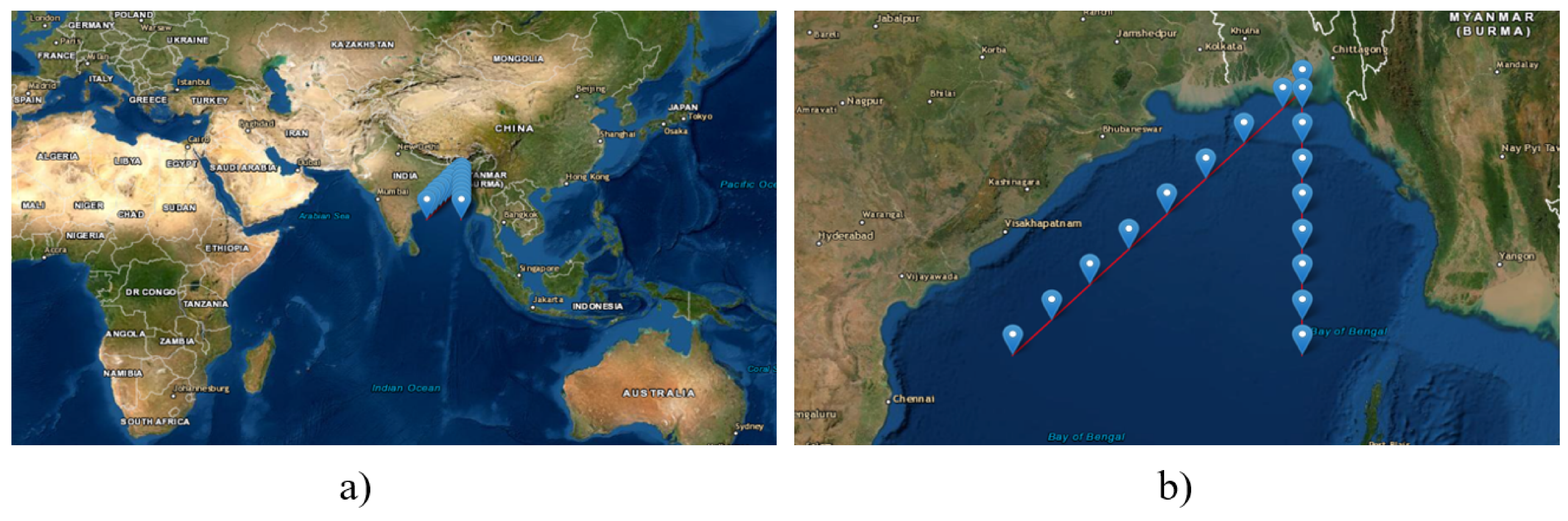
The experimental activity in proximity of the BoB 82.19 km away from the shore is considered as the initial point at a precise location of 91 E, 22.24 N. Two lines, i.e., vertical and oblique, are chosen for the computation of salinities along the way. The vertical line starts at 91 E, 14.34766 N to 91 E, 21.47852 N, covering a distance of 794.12 km. Similarly, the oblique line initiates from a position of 83.5 E, 14.34766 N to 91 E, 21.47852 N, covering a distance of 1122.873 km. Both the vertical and oblique lines are illustrated in Figure 2a,b for both the global and focused image, respectively. In addition, the exact coordinates in latitude and longitude are depicted, where Lat And Long are abbreviated for latitude and longitude, respectively, and V and O represent vertical and oblique, respectively, as depicted in

Table 2. This table presents details of the computed coordinates along the Bay of Bengal (BoB).

Serial No.	Lat, Long.(V)	Lat, Long.(O)
1	14.34766 N, 91 E	14.34766 N, 83.5 E
2	14.83153 N, 91 E	14.83153 N, 84 E
3	15.31433 N, 91 E	15.31433 N, 84.5 E
4	15.79601 N, 91 E	15.79601 N, 85 E
5	16.27655 N, 91 E	16.27655 N, 85.5 E
6	16.75592 N, 91 E	16.75592 N, 86 E
7	17.23409 N, 91 E	17.23409 N, 86.5 E
8	17.71101 N, 91 E	17.71101 N, 87 E
9	18.18668 N, 91 E	18.18668 N, 87.5 E
10	18.66195 N, 91 E	18.66195 N, 88 E
11	19.1341 N, 91 E	19.1341 N,88.5 E
12	19.60579 N, 91 E	19.60579 N, 89 E
13	20.07611 N, 91 E	20.07611 N, 89.5 E
14	20.54502 N, 91 E	20.54502 N, 90 E
15	21.0125 N, 91 E	21.0125 N, 90.5 E
16	21.47852 N, 91 E	21.47852 N, 91 E

below:

2.3. Analysis along the Yangtze River

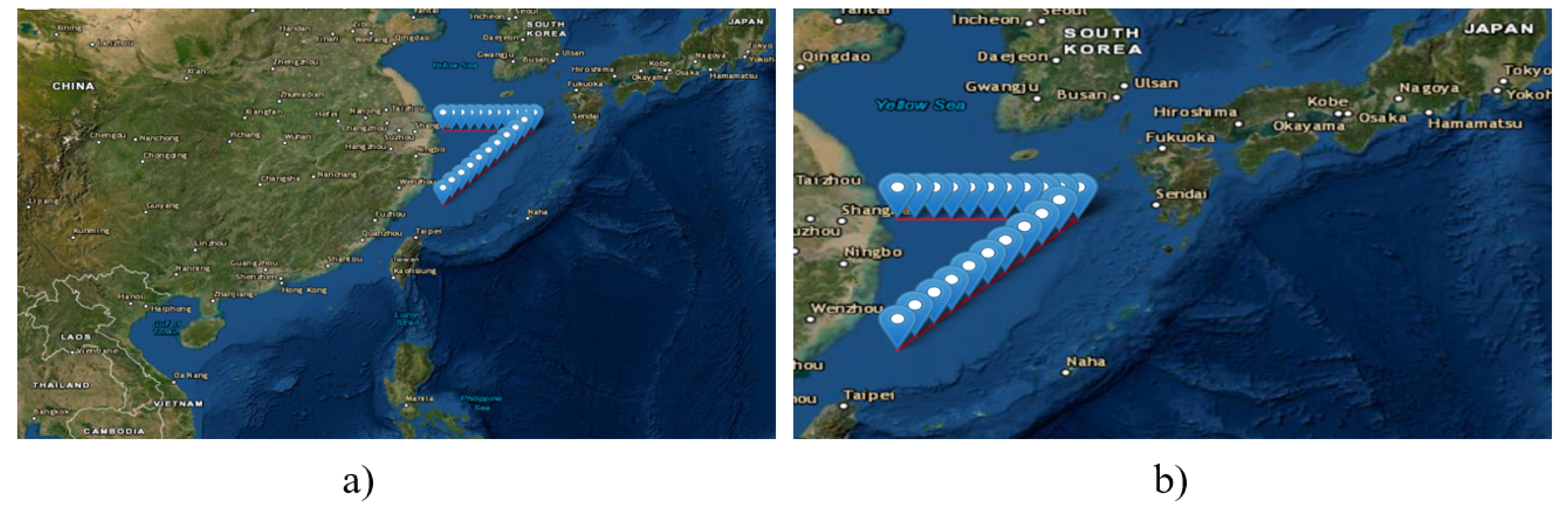
The computational activity near the Yangtze river took place 105.16 km away from the shore at the location of 121.9 E, 31.3 N. This activity was conducted by considering both horizontal and oblique dimensions. The horizontal computation of salinity initiates at 123 E, 31.3136 N to 128 E, 31.3136 N, covering a distance of 474.885 km. Similarly, the oblique line starts at 123 E, 26.94775 N to 128 E, 31.3136 N, covering a distance of 685.13 km. The locations both on the global scale and in focused form are illustrated in Figure 3a,b, respectively. Similarly, the exact coordinates in latitude and longitude are depicted, where Lat And Long are abbreviated for latitude and longitude, respectively, and H and O represent horizontal and oblique, respectively, as depicted in

Table 3. This table presents details of the computed coordinates along the Yangtze Estuary.

Serial No.	Lat, Long.(H)	Lat, Long.(O)
1	31.3136 N, 123 E	26.94775 N, 123 E
2	31.3136 N, 123.5 E	27.39258 N, 123.5 E
3	31.3136 N, 124 E	27.83562 N, 124 E
4	31.3136 N, 124.5 E	28.27686 N, 124.5 E
5	31.3136 N, 125 E	28.71628 N, 125 E
6	31.3136 N, 125.5 E	29.15387 N, 125.5 E
7	31.3136 N, 126 E	29.58959 N, 126 E
8	31.3136 N, 126.5 E	30.02345 N, 126.5 E
9	31.3136 N, 127 E	30.45541 N, 127 E
10	31.3136 N, 127.5 E	30.88546 N, 127.5 E
11	31.3136 N, 128 E	31.3136 N, 128 E

below:

3. Results

This particular section is dedicated to the results of salinity computations along the three aforementioned major freshwater influx sources, i.e., Amazon River, BoB, and Yangtze River. The results are presented in terms of salinity units, i.e., in psu, along the distance of vertical, horizontal, or oblique in km accordingly. Furthermore, the results are presented in multilayers, i.e., at 1, 3, 5, and 10 m. The results are illustrated both in 2D scales. Finally, the results are exhibited both for the maxima, i.e., maximum freshwater influx month, and the minima, i.e., minimum freshwater influx for both 2004 and 2014, in order to offer the decadal halocline analysis accordingly. The ensuing subsections represent the results at multiple locations accordingly.

3.1. The Halocline Computations along the Amazon Estuary

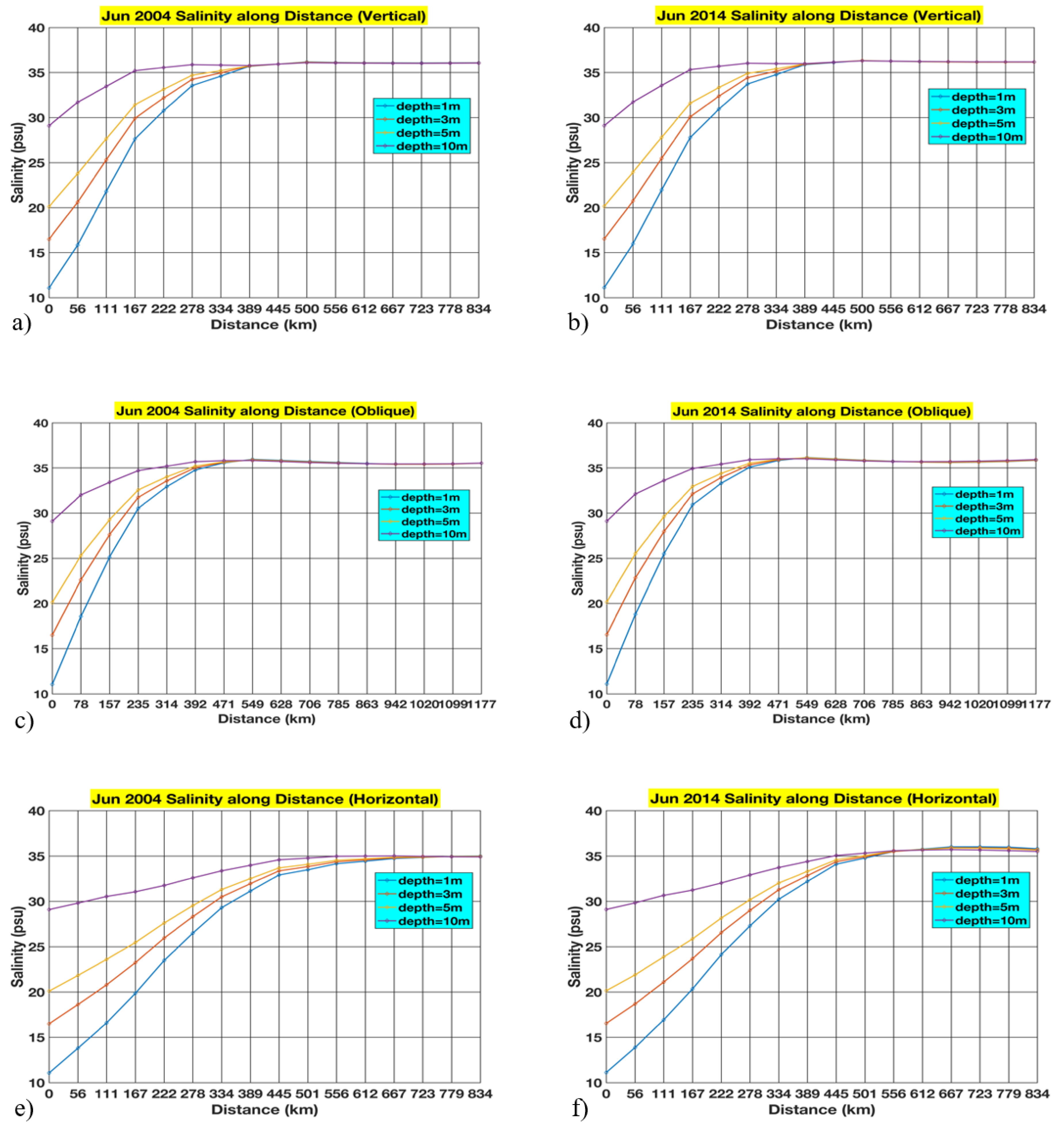
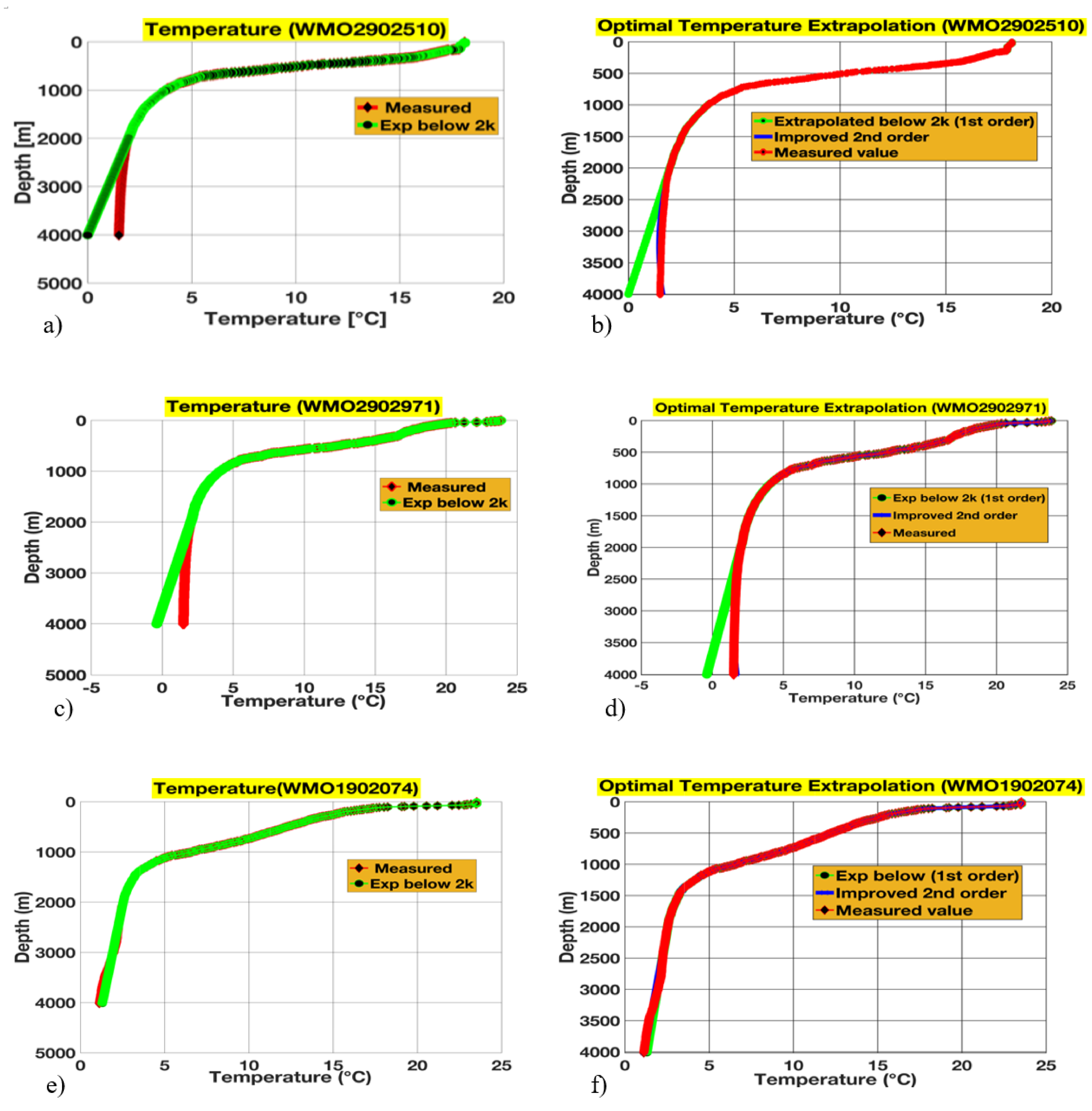
As mentioned earlier, the Amazon is responsible for the huge influx of freshwater into the Atlantic accounting for roughly 20–30% of the entire river influx in the Atlantic; thus, perturbing the haloclines in the form of salinity spikes at varying levels. Such perturbations in salinity patterns illustrate the conjoining and/or distribution of nutrients among the marine and dry land-based systems [23]. The levels for this particular study are aforementioned, i.e., 1, 3, 5, and 10 m. The salinity perturbations due to the influx of freshwater along the Amazon river are presented in 2D at multiple layers, i.e., 1, 3, 5, and 10 m, for the months of June and November in 2004, as well 2014, and illustrated in Figure 4 and Figure 5, respectively. As mentioned earlier, the analysis is based on ISAS15 datasets and the outcomes are illustrated for 2004 and 2014 vertically as (a) and (b), obliquely as (c) and (d), and horizontally as (e) and (f). The freshwater influx due to the Amazon River is three times larger during the rainy season, i.e., May and June, as compared to the dry season, i.e., December and January. This lower saline plume of the Amazon is responsible for developing a barrier layer closer to surface, which hinders mixing, enhances the surface temperature of the sea, and increases halocline stratification. This, in turn, impedes the vertical mixing of the upper high-temperature mixed layer with the low-temperature deeper ocean [15,23]. Furthermore, Junior et al. analyzed the dynamics of Zooplankton (one of the paramount groups of organisms of seaside and marine ecosystems and crucially responsible for the spread of energy via the aquatic sustenance webs of sultry estuaries) in this particular estuary of the Amazon and found that perturbations in salinity and density of varying taxa were responsible for the variations in their diversity, evenness, and richness [24,25]. The outcomes of this particular study are observed for the analysis of both June and November, and relevant perturbations in salinities are also evident. There is a slight difference in salinity deviations for both June and November during 2004, as well as 2014, as illustrated in Figure 4 and Figure 5, respectively.

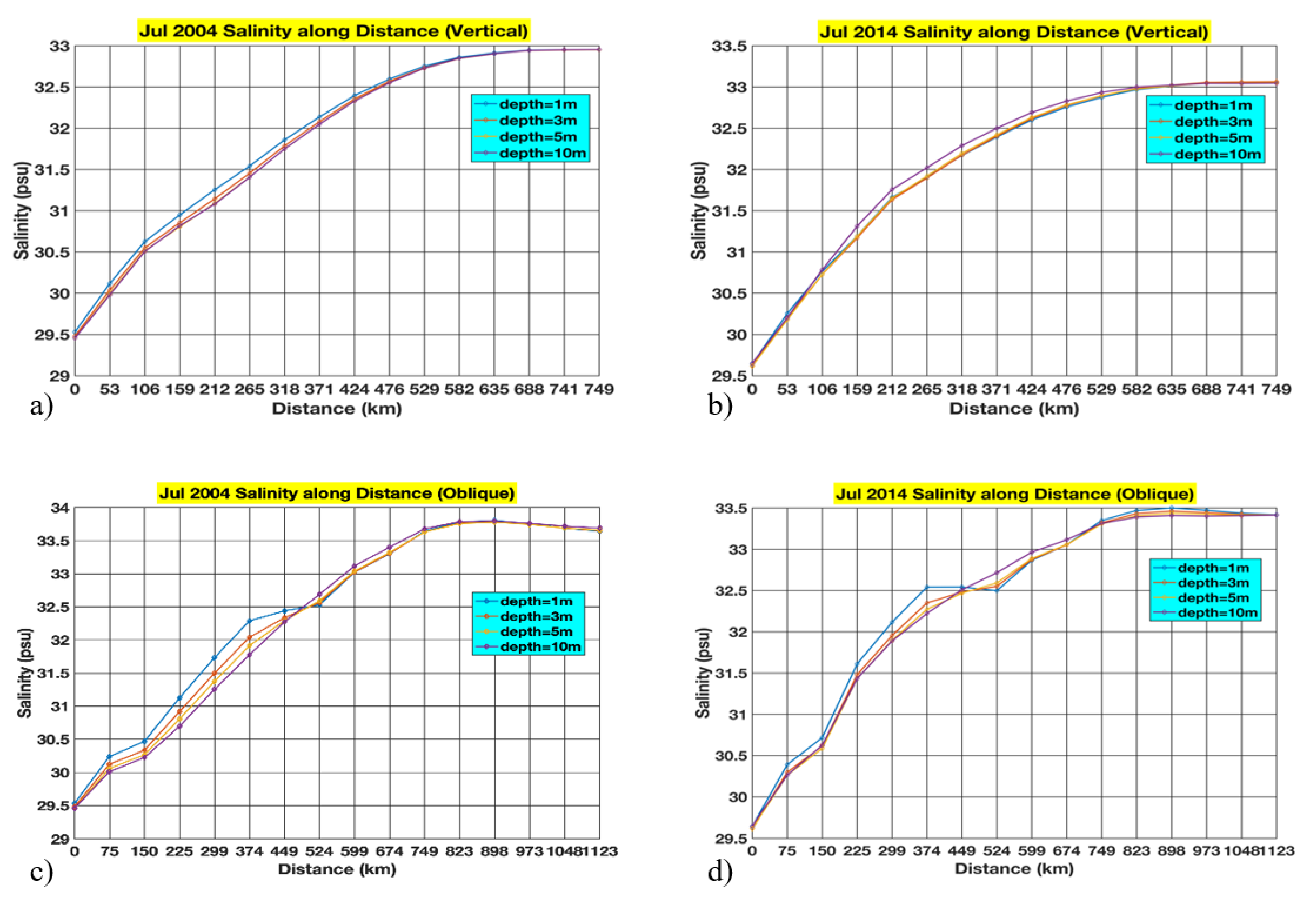
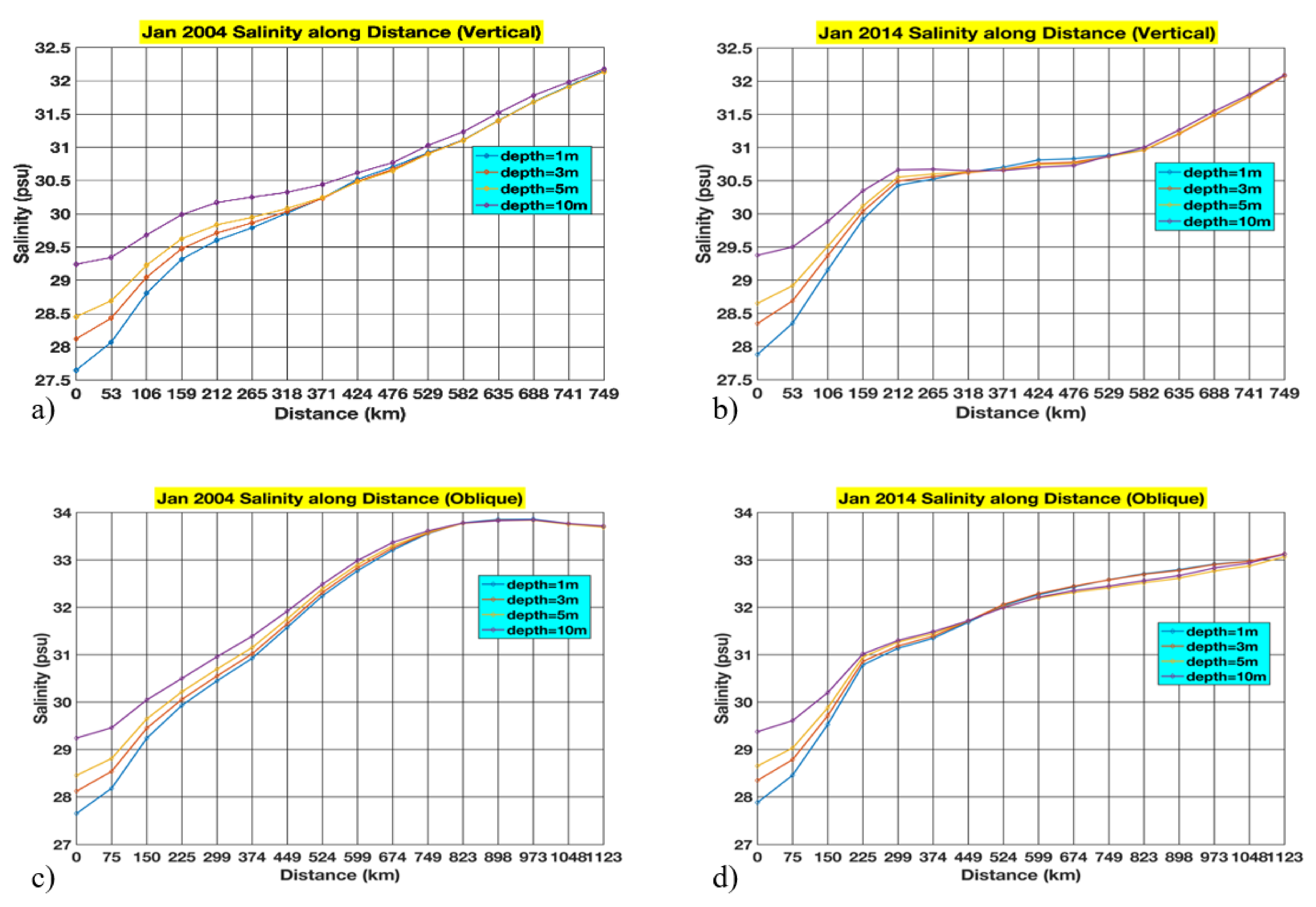
3.2. The Halocline Computations along the BoB

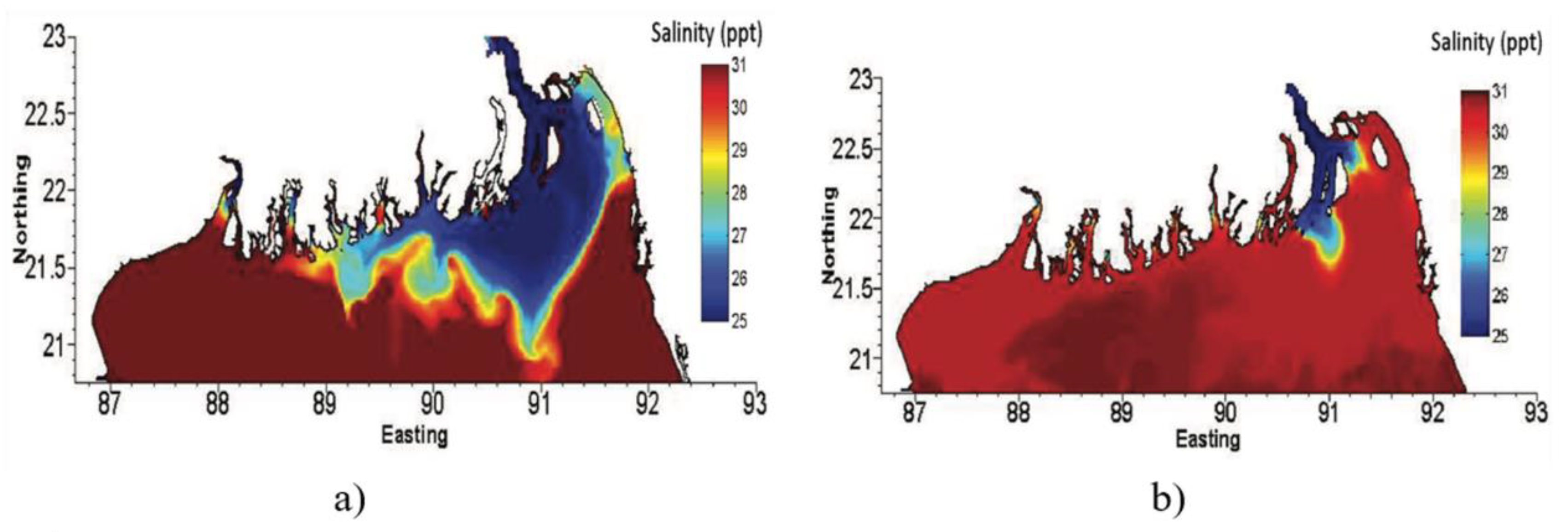
As mentioned earlier, the BoB comprises a larger area, i.e., $2.8-3.0\times {10}^6 \mathrm{sq}.\mathrm{km}$, with a maximum width of 1000 km and a peak depth of 4694 m [26,27]. This section is dedicated to measuring the halocline along this BoB both vertically starting near Bangladesh to a distance of 749 km and obliquely to a distance of 1123 km in four layers of 1, 3, 5, and 10 m by employing the ISAS15 dataset for July in 2004 and 2005, as illustrated in Figure 6, for vertical computations as (a) and (b) and oblique computations as (c) and (d), respectively. Similarly, the aforementioned comparison is conducted for the month of January in 2004 and 2014, as depicted in Figure 7, for vertical computations as (a) and (b) and oblique computations as (c) and (d), respectively. It is pertinent to mention that the surface salinities compared in Figure 6 and Figure 7 exhibit deviations from the established norms of the BoB as established in the literature. In this regard, Vinayachandran et al. categorically ascribed the freshwater influxes/sinks and the subsequent distribution of the ensuing lower- or higher-salinity water by oceanic currents to the seasonal balancing of salinity in the Indian Ocean [28]. Furthermore, Hussain et al. explicitly illustrated the relative surface salinities during both monsoon and winter, which are depicted in Figure 8a,b, respectively [29]. Moreover, the deviations within the months of July and January show deviations for the years 2004 and 2014. These entire deviations or anomalies may be due to multiple reasons, i.e., mentioned by Mahadevan et al., who evaluated the rate of water becoming saline along the trajectory as it leaves the northern bay [30], and by Banerjee who analyzed surface water salinity perturbations of Indian Sundarbans on the decadal scale as a prospective criterion of climate change. Such climatological perturbations have enhanced during the last two decades due to the global rise in temperature, removal of glacial land ice from the Gangotri Glacier of the Himalayan ranges, influxes of the Farakka embankment, and an increase in the sea level. In this regard, remarkable continuing discrepancies are observed while monitoring salinity for a period of 23 years, i.e., from 1990 to 2012 [31]. Similarly, salinity perturbations in the BoB away from the shores may be either due to the interchangeability of waters among the Arabian Sea and BoB as the Arabian Sea appears to be saltier due to its proximities to the couple of high-salinity seas, i.e., Red Sea and the Persian Gulf, or due to the influx of eastern rivers of Burma, i.e., Irrawaddy and Salween, which discharge $430\times {10}^9$ and $300 \times {10}^9{\mathrm{m}}^3{\mathrm{year}}^{-1}$, respectively [14,28]. In this regard, an aforementioned ingenious method based on least squares is proposed at the end of this section to assess this particular region on a wider spatiotemporal coverage for both halocline and thermocline analysis. In situ data from varying parts of global oceans are obtained with the help of deep Argo floats, and extrapolations are conducted to the nearest identical values. Such extrapolations conjoining core and deep Argo programs will help to assess this region with more conviction as a future course of action.

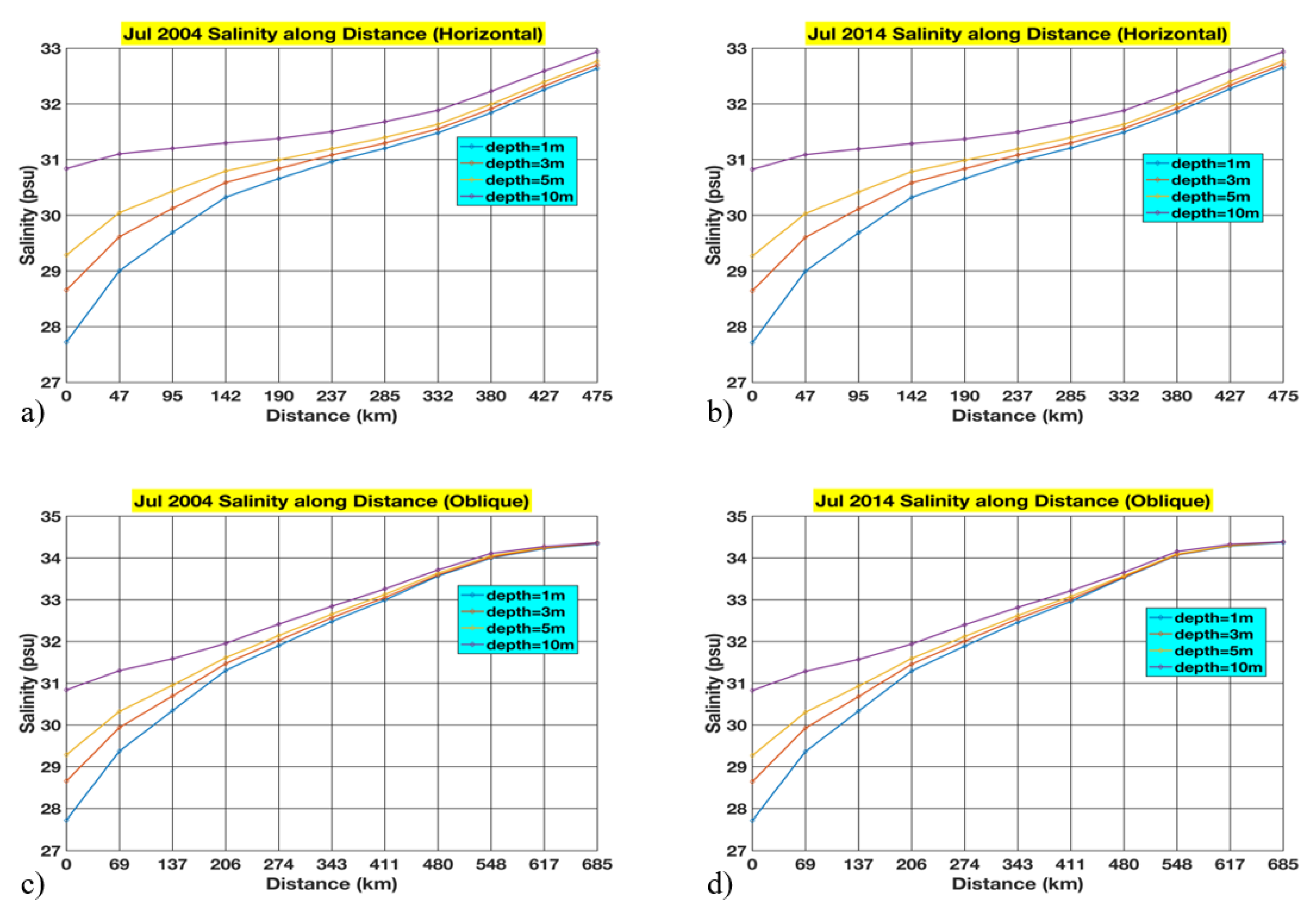
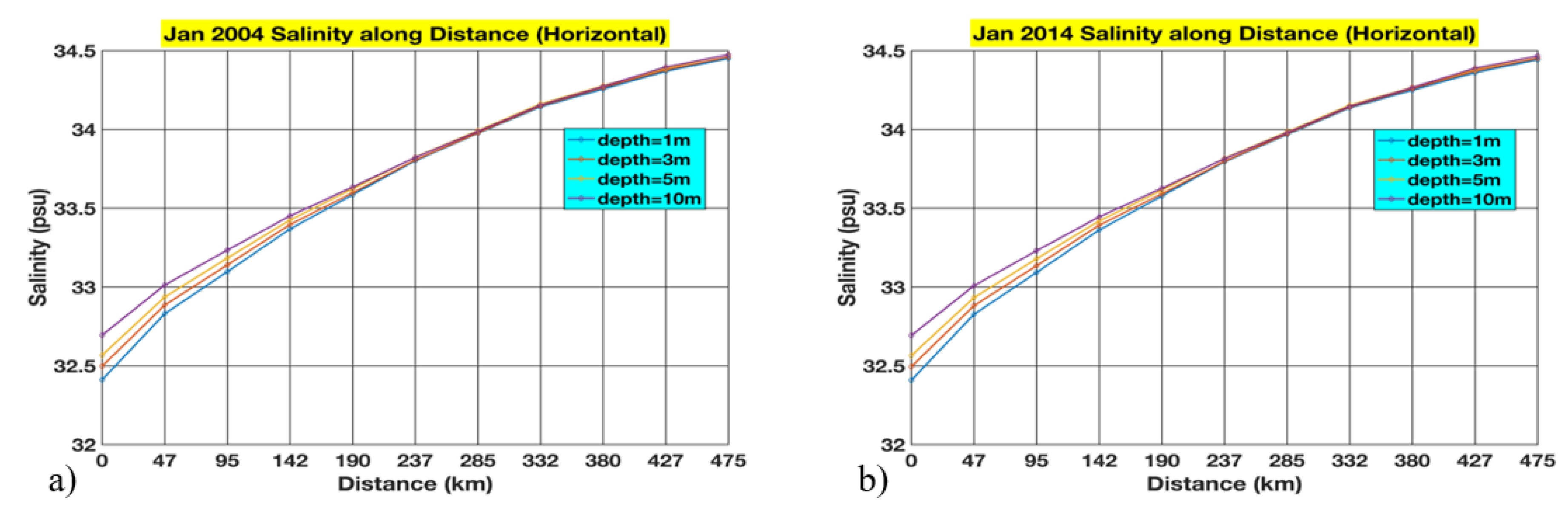
3.3. The Halocline Computations along the Yangtze Estuary

As mentioned earlier, Yangtze is the longest river in China and constitutes the biggest estuary by comprising three bifurcations and four channels into the East China Sea [21]. Sun et al. undertook the environmental flow depending on the salinity objectives for the Yangtze estuary of China to analyze the effects of varying freshwater discharge on the estuarine ecosystem. They mentioned strong correlations between freshwater influx and the salinity gradient, as well as correlation between salinity and a large variety of kinds of biological productivity [32]. This particular section of our study is dedicated to compute and compare haloclines for the Yangtze Estuary during the months of July in 2004 and 2014, as well as January in 2004 and 2014, as illustrated in Figure 9 and Figure 10, respectively. These comparative analyses are conducted horizontally to a distance of 475 km from the estuary and obliquely 685 km from the initial observation location. The halocline comparisons are exhibited in five layers as done in previous experimentations, i.e., 1, 3, 5, and 10 m. The outcomes in Figure 9 and Figure 10are illustrated for horizontal computations as (a) and (b) and oblique computations as (c) and (d). The outcomes illustrated in Figure 9 and Figure 10 exhibit the salinity deviations according to the literature regarding the freshwater influx during the months of July and January, respectively [21,33]. Moreover, a slight difference is observed between 2004 and 2014 comparisons in the months of both July and January.

The aforementioned method proposed to ascertain the BoB both on the temporal and spatial scale for future course of action is presented mathematically. As mentioned earlier, this proposed method is based on the least squares method [22]. This method ingeniously conjoins datasets from core Argo and deep Argo in order to extrapolate and depends on in situ deep ocean values either from deep Argo or from any other sensing source. The data are depicted in Equation (1) below, where x illustrates the salinities, temperatures, and SSPs in psu, °C, and m/s, respectively, whereas y demonstrates the depth in meters, and $i=1,2,3,\dots ,n$.

$$D=\left(x_i,y_i\right)$$

(1)

In order to employ polynomials for curve fitting, we have

$$f\left(x\right)={{\displaystyle \sum }}_{j=0}^m{k}_j{x}^j.$$

(2)

Here, $k=\left(k_0,k_1,\dots ,k_m\right)$ are the desired design parameters. Then, we have

$$R\left(k\right)={{\displaystyle \sum }}_{i=1}^n{\left[y_i-f\left(x_i\right)\right]}^2.$$

(3)

In order to acquire the most desirable fitting, classical least squares is applied [34]. By differentiating each side, we come up with

$$\frac{\partial R\left(\kappa \right)}{\partial k_j}=-2{{\displaystyle \sum }}_{i=1}^n\left[y_i-f\left(x_i\right)\right]x_i^j=0, j=0\dots m.$$

(4)

Now, substituting Equation (2) into Equation (4), we have

$${{\displaystyle \sum }}_{i=1}^n{{\displaystyle \sum }}_{l-0}^m{k}_l{x}_i^{l+j}={{\displaystyle \sum }}_{i=1}^n{y}_i{x}_i^j$$

(5)

which is of the form $A{\kappa }^{*}=b$ where $A=\left\{a_{ij}\right\}$ with $a_{ij}={\displaystyle \sum }_{l=0}^m{x}_i^{l+j}$ and $b=\left\{b_j\right\}$ with $b_j=\{{\displaystyle \sum }_{i=1}^n{y}_i{x}_i^j$, $j=0,\dots ,m$ and $i=1,\dots ,n$.

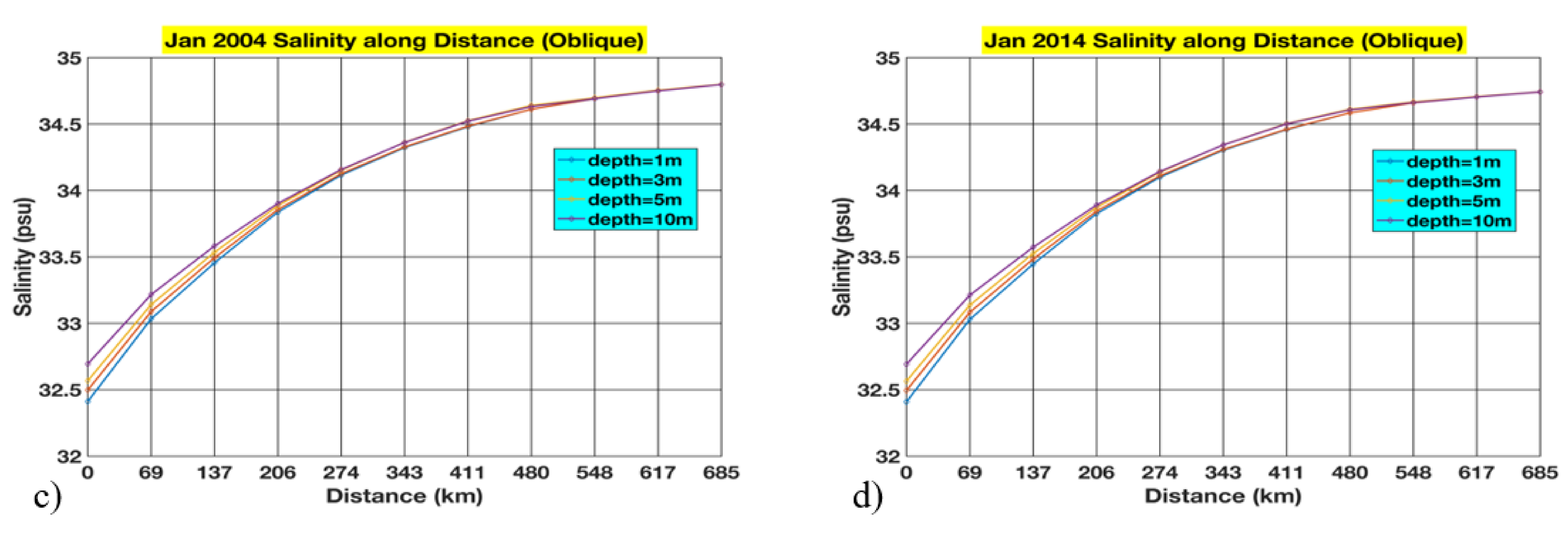
The $m$ and $n$ can be chosen freely, and certain values are selected for them to acquire extrapolations of salinities, temperatures, and SSPs that are nearly analogous to the in-situ values of the Deep Argo buoys. In this regard, $m$ was set to 1 in the initial stages for extrapolations with different values of $n$, which were 32, 78, and 14 for the corresponding buoys, i.e., World Meteorological identification (WMO) WMO2902510, WMO2902971, and WMO1902074, respectively, as detailed in

Table 4. The buoys with vertical profiles up to depths of 4000 m.

Float Identity	Cycle Number	Date	Lat and Long	Location
WMO2902510	24	2 March 2014	30.447° N, 146.004° E	Pacific Ocean
WMO2902971	08	12 May 2016	29.566° N	Pacific Ocean
WMO1902074	08	11 April 2016	28.998° S, 52.16° E	Indian Ocean

, and their results are exhibited in Figure 11a,c,e, respectively. Then, in order to rectify the anomalies shown for the value of $m$ equal to 1 in Figure 11a,c,e, $m$ was changed to 2 for the case of the second-order polynomial, and the outcomes almost identical to the in situ values are illustrated in Figure 11b,d,f, respectively.

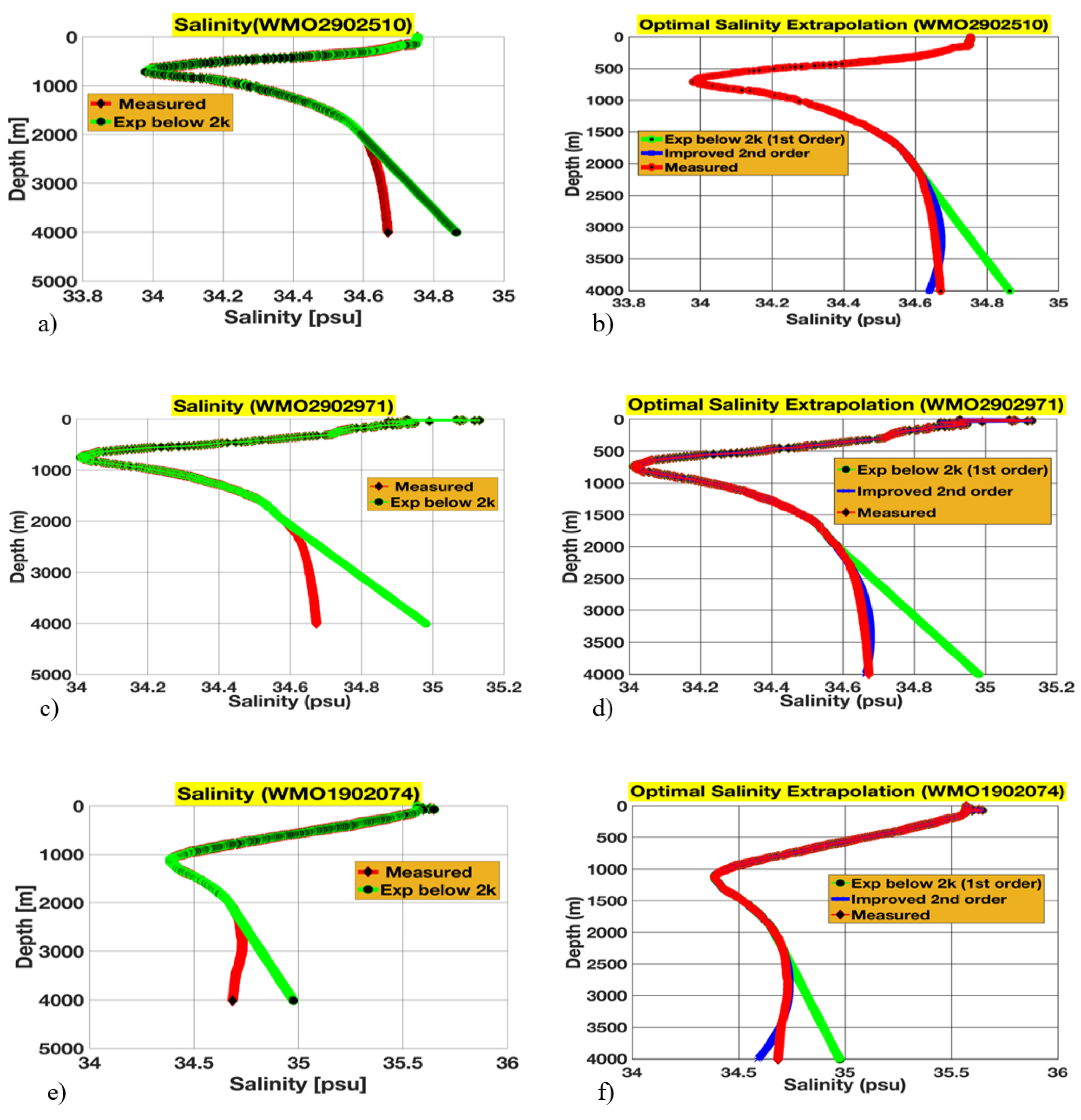
The salinity in the ocean is a sign of variations in the worldwide hydrological cycle and extensive climate perturbation. The spread of salt in the ocean along with its temporal discrepancy is crucial for comprehending Earth’s weather. The thermohaline circulation along with the spread of heat and mass is critically dependent on the salinity of the ocean. In addition, temperature along with salinity and pH are crucial to the existence of the majority of marine flora and fauna and, hence, are critical parameters for the observation of water [23,35]. In this regard, temperature is extrapolated below 2000 m analogous to the extrapolations of salinity conducted for the Argo floats presented in Table 4. These temperature extrapolations are illustrated in Figure 12a,c,e for the aforementioned basic first-order method for Argo floats of WMO2902510, WMO2902971, and WMO1902074, respectively. Similarly, the improved second-order polynomial is employed to rectify the anomalies, as illustrated in Figure 12b,d,f, respectively. As mentioned earlier, such extrapolations for both salinity and temperature may pave the way for the broader spatiotemporal coverage of assessing varying regions of the ocean by taking into consideration the core as well as deep Argo programs.

In order to compute the SSPs for three deep Argo buoys, i.e., WMO5905738, WMO5905739, and WMO5905740 are detailed in

Table 5. The buoys from the Pacific Ocean.

Float Identity	Cycle	Lat, Long.	Date	Time
WMO5905738	20	22.6443° N, 158.6656° W	19 July 2018	11:52:11
WMO5905739	20	22.8836° N, 158.7888° W	3 July 2018	04:03:52
WMO5902521	20	12.0588° N, 154.0620° W	19 September 2018	07:54:23

by employing the Del Grosso equation (1974), which employs the vertical profiles of both salinities and temperatures of the aforementioned buoys. This particular equation was reassessed by Zhu and Wong (1995) in order to adjust according to the new International Temperature Scale of 1990, and is given as [36,37]:

$$c\left(S,T,P\right)= C_{000}+\Delta C_T+\Delta C_S+\Delta C_P+\Delta C_{STP}$$

(6)

$$\Delta C_T\left(T\right)=C_{T1}T+C_{T2}{T}^2+C_{T3}{T}^3$$

(7)

$$\Delta C_S\left(S\right)=C_{S1}S+C_{S2}{S}^2$$

(8)

$$\Delta C_P\left(P\right)=C_{P1}P+C_{P2}{P}^2+C_{P3}{P}^3$$

(9)

$$\Delta C_{STP}\left(S,T,P\right)=C_{TP}TP+C_{T3P}{T}^{3}P+C_{TP2}T{P}^2+C_{T2P2}{T}^2{P}^2+C_{TP3}T{P}^3$$

(10)

$$C_{ST}ST+C_{ST2}S{T}^2+C_{STP}STP+C_{S2TP}{S}^{2}TP+C_{S2P2}{S}^2{P}^2$$

(11)

T represents the temperature in °C, S exhibits the salinity in Practical Salinity Units, and P illustrates the pressure in kg/cm². The range of validity for temperature is 0 to 30 °C, whereas that for salinity is 30 to 40 parts per thousand, and that for pressure is 0 to 1000 kg/cm², where 100 kPa = 1.019716 kg/cm².

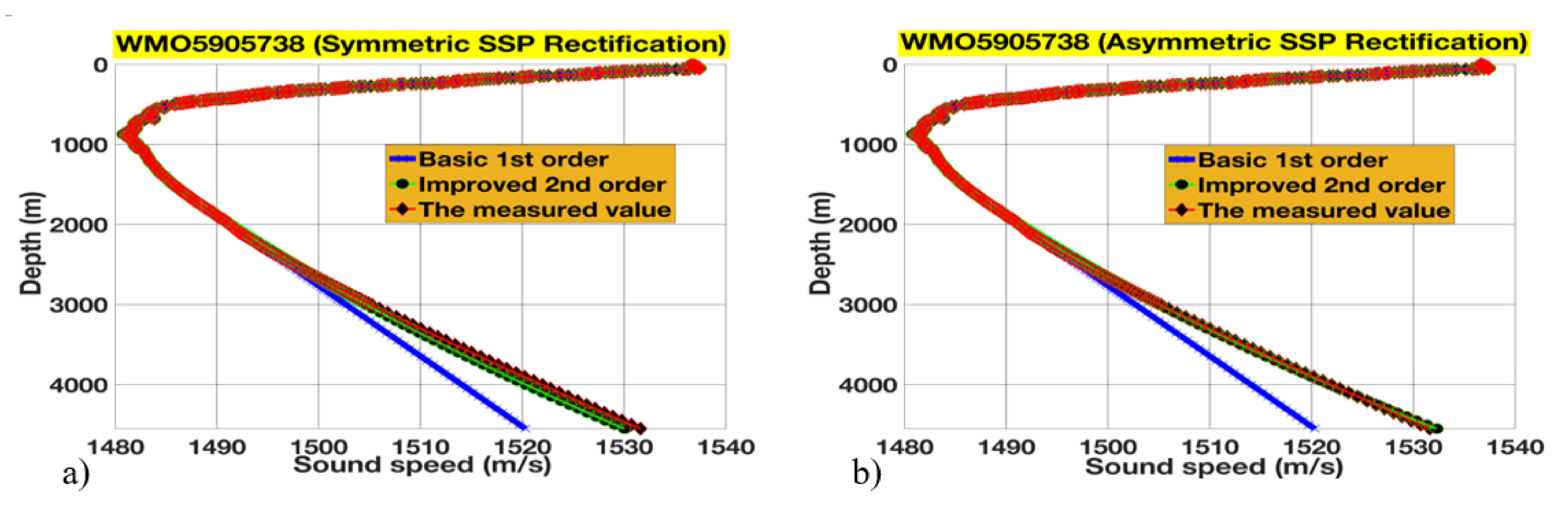
The SSPs obtained from the above computations are extrapolated for the buoys mentioned in Table 5 in a symmetrical way by keeping the values of both $m$ and $n$ the same (i.e., $m=2$ and $n=40$), as shown in Figure 13a,c,e. Similarly, the asymmetric extrapolations were conducted for these buoys as $m$ = 2 and $n$ = 46 for WMO5905738, $m$ = 3 and $n$ = 68 for WMO5905739, and $m$ = 2 and $n$ = 37 for WMO5905740, as illustrated in Figure 13b,d,f, respectively. It is explicitly evident that by changing the values of $m$, as well as $n$, i.e., by correcting asymmetrically, the acquired corrected computations became nearly identical to the in situ-measured values of the buoys.

4. Conclusions

The study explains the varying effects of salinity perturbations due to major influxes of freshwater into the respective seas. In this regard, the study ingeniously employs the datasets of ISAS15 to ascertain the halocline perturbations along the estuaries of three major sources of freshwater influxes, i.e., in proximity of the Amazon, BoB, and Yangtze River. The study proceeds to ascertain the comparative analyses of halocline perturbations in maxima and minima months, i.e., maximum influx and minimum influx of freshwater both in 2004 and in 2014. The computations along the Amazon and Yangtze proved to be in accordance with the documented literature data. However, the deviations were computed for the months of July and January in proximity of the BoB during both 2004 and 2010. The study concludes by presenting and employing an ingenious method that is capable of extrapolating salinities, temperatures, and SSPs to deeper depths by its pioneer application of a basic first-order technique based on the least squares method, which extrapolates the Argo data to deeper depths. Then, this method is adjusted to employ the second-order polynomial, which rectifies the anomalies in the extrapolation for the basic first-order method. This particular method lays the foundation to counter and/or rectify the deviations identified in the BoB. In addition, it offers a broader spatiotemporal investigation platform to assess varying regions on an almost global scale after conjoining it with the ISAS tool for the future course of action.

References

- Cloern, J.E.; Jassby, A.D.; Schraga, T.S.; Nejad, E.; Martin, C. Ecosystem variability along the estuarine salinity gradient: Examples from long-term study of San Francisco Bay. Limnol. Oceanogr. 2017, 62, S272–S291. [Google Scholar] [CrossRef] [Green Version]
- Kennedy, V.S.; Twilley, R.R.; Kleypas, J.A.; Cowan, J.H., Jr.; Hare, S.R. Coastal and Marine Ecosystems & Global Climate Change: Potential Effects on U.S. Resources; Pew Center on Global Climate Change: Arlington, VA, USA, 2002. [Google Scholar]
- Wheatly, M.G. Integrated Responses to Salinity Fluctuations. Amer. Zool. 1988, 28, 65–77. [Google Scholar] [CrossRef]
- Durack, P. Ocean Salinity and the Global Water Cycle. Oceanography 2015, 28, 20–31. [Google Scholar] [CrossRef] [Green Version]
- LloveL, W.; Purkey, S.G.; Meyssignac, B.; Blazquez, A.; Kolodziejczyk, N.; Bamber, J.L. Global ocean freshening, ocean mass increase and global mean sea level rise over 2005–2015. Sci. Rep. 2019, 9, 1–10. [Google Scholar] [CrossRef]
- Freeland, H. Argo—A Decade of Progress. In Proceedings of the OceanObs’09: Sustained Ocean Observations and Information for Society, Venice, Italy, 21–25 September 2009; WPP-306; Hall, J., Harrison, D.E., Stammer, D., Eds.; ESA Publication WPP-306: Auckland, New Zealand, 2009. [Google Scholar] [CrossRef] [Green Version]
- Kolodziejczyk, N.; LloveL, W.; Portela, E. Interannual Variability of Upper Ocean Water Masses as Inferred From Argo Array. J. Geophys. Res. Oceans 2019, 124, 6067–6085. [Google Scholar] [CrossRef]
- Roemmich, D.; Alford, M.H.; Claustre, H.; Johnson, K.; King, B.; Moum, J.; Oke, P.; Owens, W.B.; Pouliquen, S.; Purkey, S.; et al. On the Future of Argo: A Global, Full-Depth, Multi-Disciplinary Array. Front. Mar. Sci. 2019, 6, 439. [Google Scholar] [CrossRef] [Green Version]
- Schmid, C.; Molinari, R.L.; Sabina, R.; Daneshzadeh, Y.-H.; Xia, X.; Forteza, E.; Yang, H. The Real-Time Data Management System for Argo Profiling Float Observations. J. Atmos. Ocean. Technol. 2007, 24, 1608–1628. [Google Scholar] [CrossRef]
- Gaillard, F.; Reynaud, T.; Thierry, V.; Kolodziejczyk, N.; Von Schuckmann, K. In Situ–Based Reanalysis of the Global Ocean Temperature and Salinity with ISAS: Variability of the Heat Content and Steric Height. J. Clim. 2016, 29, 1305–1323. [Google Scholar] [CrossRef]
- Thierry, V.; Kolodziejczyk, N.; Prigent, A. T,S,O2 EOV: T, S and Oxygen Syntheses and Impact of AtlantOS Observations. 2019. Available online: https://www.atlantos-h2020.eu/download/deliverables/AtlantOS_D7.12.pdf (accessed on 28 June 2020).
- Kolodziejczyk, N.; Reverdin, G.; Desbruyeres, D. Contribution to the ICES Report on Ocean Climate: North Atlantic Ocean in 2017, National Report: France. June 2018. Available online: https://archimer.ifremer.fr/doc/00481/59296/61988.pdf (accessed on 29 June 2020).
- Gonzalez-Pola, C.; Larsen, K.M.H.; Fratantoni, P.; Beszczynska-Moller, A. (Eds.) ICES Report on Ocean Climate 2018. ICES Cooperative Research Report No. 349. 122 pp. 2019. Available online: https://doi.org/10.17895/ices.pub.5461 (accessed on 2 July 2020).
- Dagg, M.; Benner, R.; Lohrenz, S.; Lawrence, D. Transformation of dissolved and particulate materials on continental shelves influenced by large rivers: Plume processes. Cont. Shelf Res. 2004, 24, 833–858. [Google Scholar] [CrossRef]
- Giffard, P.; Llovel, W.; Jouanno, J.; Morvan, G.; Decharme, B. Contribution of the Amazon River Discharge to Regional Sea Level in the Tropical Atlantic Ocean. Water 2019, 11, 2348. [Google Scholar] [CrossRef] [Green Version]
- Masson, S.; Delecluse, P. Influence of the Amazon River runoff on the tropical Atlantic. Phys. Chem. Earth Part B Hydrol. Oceans Atmos. 2001, 26, 137–142. [Google Scholar] [CrossRef]
- Kang, Y.-M.; Pan, D.; Bai, Y.; He, X.; Chen, X.; Chen, C.-T.A.; Wang, D. Areas of the global major river plumes. Acta Oceanol. Sin. 2013, 32, 79–88. [Google Scholar] [CrossRef]
- Mohanty, P.K.; Pradhan, Y.; Nayak, S.R.; Panda, U.S.; Mohapatra, G.N. Sediment Dispersion in the Bay of Bengal. In Monitoring and Modelling Lakes and Coastal Environments; Springer: Dordrecht, The Netherlands, 2008. [Google Scholar] [CrossRef]
- Kay, S.; Caesar, J.; Janes, T. Marine Dynamics and Productivity in the Bay of Bengal. In Ecosystem Services for Well-Being in Deltas; Springer International Publishing: Cham, Switzerland, 2018. [Google Scholar] [CrossRef] [Green Version]
- Dai, S.; Lu, X. Sediment load change in the Yangtze River (Changjian): A review. Geomorphology 2014, 215, 60–73. [Google Scholar] [CrossRef]
- Xu, Z.; Ma, J.; Wang, H.; Hu, Y.; Yang, G.; Deng, W. River Discharge and Saltwater Intrusion Level Study of Yangtze River Estuary, China. Water 2018, 10, 683. [Google Scholar] [CrossRef] [Green Version]
- Steven, J.M. The Methods of Least Squares. Mathematics Department Brown University, Providence, RI, 02912. Available online: https://web.williams.edu/Mathematics/sjmiller/public_html/BrownClasses/54/handouts/MethodLeastSquares.pdf (accessed on 1 September 2020).
- Tyaquiçã, P.; Veleda, D.; Lefèvre, N.; Araujo, M.; Noriega, C.; Caniaux, G.; Servain, J.; Silva, T. Amazon Plume Salinity Response to Ocean Teleconnections. Front. Mar. Sci. 2017, 4, 250. [Google Scholar] [CrossRef] [Green Version]
- Júnior, A.N.D.S.; Magalhães, A.; Pereira, L.C.C.; Rauquírio, M.D.C. Zooplankton dynamics in a tropical Amazon estuary. J. Coast. Res. 2013, 1230–1235. [Google Scholar] [CrossRef]
- Costa, R.M.; Leite, N.R.; Pereira, L.C.C. Mesozooplankton of the Curuca Estuary (Amazon Coast, Brazil). J. Coast. Res. 2009, 400–404. [Google Scholar]
- Sarma, K.V.L.N.S.; Ramana, M.V.; Subrahmanyam, V.; Krishna, K.S.; Ramprasad, T.; Desa, M. Morphological features in the Bay of Bengal. J. Ind. Geophys. Union 2000, 4, 185–190. [Google Scholar]
- Britannica Website. Available online: https://www.britannica.com/place/Bay-of-Bengal (accessed on 3 September 2020).
- Vinayachandran, P.N.; Nanjundiah, R.S. Indian Ocean sea surface salinity variations in a coupled model. Clim. Dyn. 2009, 33, 245–263. [Google Scholar] [CrossRef]
- Hussain, M.A.; Islam, A.K.M.S.; Hossain, M.A.; Hoque, T. Assessment of Salinity Distributions and Residual Currents at the Northern Bay of Bengal considering Climate Change Impacts. Int. J. Ocean Clim. Syst. 2012, 3, 173–186. [Google Scholar] [CrossRef] [Green Version]
- Mahadevan, A.; Jaeger, G.S.; Freilich, M.A.; Omand, M.; Shroyer, E.; Sengupta, D. Freshwater in the Bay of Bengal: Its Fate and Role in Air-Sea Heat Exchange. Oceanography 2016, 29, 72–81. Available online: www.jstor.org/stable/24862671 (accessed on 14 September 2020). [CrossRef] [Green Version]
- Banerjee, K. Decadal Change in the Surface Water Salinity Profile of Indian Sundarbans: A Potential Indicator of Climate Change. J. Mar. Sci. Res. Dev. 2013, 1. [Google Scholar] [CrossRef]
- Sun, T.; Yang, Z.; Shen, Z.; Zhao, R. Environmental flows for the Yangtze Estuary based on salinity objectives. Commun. Nonlinear Sci. Numer. Simul. 2009, 14, 959–971. [Google Scholar] [CrossRef]
- Zhu, J.; Wu, H.; Li, L. Hydrodynamics of the Changjiang Estuary and Adjacent Seas. In Estuaries of the World; Springer Science and Business Media LLC: Berlin/Heidelberg, Germany, 2015; pp. 19–45. [Google Scholar]
- Bretscher, O. Linear Algebra with Applications, 3rd ed.; Prentice Hall: Upper Saddle River, NJ, USA, 2004. [Google Scholar]
- pH, Salinity and Temperature. Available online: https://sfyl.ifas.ufl.edu/media/sfylifasufledu/miami-dade/documents/sea-grant/Temperature,-Salinity-and-pH.pdf (accessed on 1 October 2020).
- Underwater Acoustics: Technical Guides—Speed of Sound in Sea-Water. National Physical Laboratory, Teddington, Middlesex, UK, TW11 0LW. Available online: http://resource.npl.co.uk/acoustics/techguides/soundpurewater/speedpw.pdf (accessed on 4 September 2020).
- Wong, G.S.K.; Zhu, S.-M. Speed of sound in seawater as a function of salinity, temperature, and pressure. J. Acoust. Soc. Am. 1995, 97, 1732–1736. [Google Scholar] [CrossRef]
Figure 1.
The experimental activity area illustrating vertical, horizontal, and oblique computations in proximity of the Amazon Estuary for halocline perturbations both globally in (a), as well as in focused form as (b) (Courtesy: https://earthexplorer.usgs.gov).
Figure 2.
The area of experimental computations illustrating vertical and oblique dimensions in the BoB both globally in (a) and in focused form as (b) (Courtesy: https://earthexplorer.usgs.gov).
Figure 3.
The area of experimental computations illustrating vertical and oblique dimensions in proximity of the Yangtze Estuary both globally in (a) and in focused form as (b) (Courtesy: https://earthexplorer.usgs.gov).
Figure 4.
Comparative analysis of the halocline for multiple layers, i.e., 1, 3, 5, and 10 m, for 2004 and 2014 in the month of June near the Amazon estuary for vertical stretches as (a,b), oblique stretches as (c,d), and horizontal stretches as (e,f).
Figure 5.
Comparative analysis of the halocline for multiple layers, i.e., 1, 3, 5, and 10 m, for 2004 and 2014 in the month of November near the Amazon estuary for vertical stretches as (a,b), oblique stretches as (c,d), and horizontal stretches as (e,f).
Figure 6.
Comparative analysis of the halocline for multiple layers, i.e., 1, 3, 5, and 10 m, for 2004 and 2014 in the month of July in proximity of the BoB for vertical stretches as (a,b) and oblique stretches as (c,d).
Figure 7.
Comparative analysis of the halocline for multiple layers, i.e., 1, 3, 5, and 10 m, for 2004 and 2014 in the month of January in proximity of the BoB for vertical stretches as (a,b) and oblique stretches as (c,d).
Figure 8.
The surface salinity illustrations in the BoB in year 2000 with (a) depicting the perturbations in monsoon, whereas (b) indicates the salinities during winter (courtesy: Hussain et al. 2012).
Figure 9.
Comparative analysis of the halocline for multiple layers, i.e., 1, 3, 5, and 10 m, for 2004 and 2014 in the month of July near Yangtze estuary for vertical stretches as (a,b), oblique stretches as (c,d).
Figure 10.
Comparative analysis of the halocline for multiple layers, i.e., 1, 3, 5, and 10 m, for 2004 and 2014 in the month of January near Yangtze estuary for vertical stretches as (a,b), oblique stretches as (c,d).
Figure 11.
The application of the basic first-order method to extrapolate the salinities below 2000 m is illustrated in (a,c,e). Similarly, the improved second-order polynomial is employed to further rectify the anomalies, and the improved results are presented in (b,d,f).
Figure 12.
Extrapolating temperature by employing basic first-order method below 2000 m as illustrated in (a,c,e). The improved second-order polynomial is employed to rectify the anomalies, and the improved outcomes are depicted as (b,d,f).
Figure 13.
The sound speed profiles (SSPs) from symmetric extrapolations were rectified by asymmetric extrapolation, resulting in an improvement of ~2 m/s to become almost identical (a,b). Similarly, an improvement was observed from ~7 m/s to negligible difference (c,d). Finally, a difference of ~5 m/s was improved to ~1 m/s, as illustrated in (e,f), respectively.