An Analytical Study on Wave-Current-Mud Interaction

Abstract

This study aims at providing analytical investigations to the first and second-order on the wave–current–mud interaction problem by applying a perturbation method. Direct formulations of the wave–current–mud interaction could not be found in the literature. Explicit formulations for the particle velocity, dissipation rates, and phase shift in the first order and the mass transport in the second-order have been obtained. The findings of the current study confirmed that by an increase in the current velocity (e.g., moving from negative to positive values of current velocity), the dissipation rates and mud (instantaneous and mean) velocity decrease. The proposed assumption of a thin mud layer (boundary layer assumption) matches with the laboratory data in the mud viscosity of the orders of (0.01 N/m²) in both wave dissipation and mud mass transport leading to small ranges of discrepancies. The results from the newly proposed model were compared with the measurements and the results of an existing model in the literature. The proposed model showed better agreements in simulating the mud (instantaneous and mean) velocity compared to the existing one.

1. Introduction

Phenomena relevant to the water–sediment systems are of great importance in the coastal zones all over the world. Therefore, water–sediment interaction should be studied from different perspectives, e.g., coastal protection, land reclamation, and water quality management [1]. Some parts of the coasts including estuaries and mouths of large rivers are mainly covered by the soft mud (Lousiana coast [2]; Brazil [3]; South Korea [4]; and Iran [5]). The current exists in most of the cases in the fields of water-mud systems, especially in the confluences of large rivers and estuaries (e.g., Ems estuary [6]; Southampton water estuary [7]). The current substantially affects the two major aspects of wave mud interaction: wave attenuation, and mud mass transport, which are highly influential in the coastal systems in the environmental, engineering, and management aspects [1]. While both wave attenuation and mud transport affect the designing of the harbors and ports [8], the mud mass transport may also cause some environmental issues by carrying the pollutant species toward the coasts [9]. The current influences a wave field by shifting the frequency and changing the amplitude, and it plays a significant role in the development of the waves of unusual character. Current can also refract waves, change the direction of wave propagation, and consequently affect the nearshore hydrodynamics [10].

Wave–mud interactions have been widely studied in several aspects including wave height attenuation ([11,12,13]), mud mass transport as the bed load ([8,9,14,15,16] among many others), stratified two-phase flows ([12,17]), and, suspended load (e.g., the most recent ones are [18,19]). Many analytical and experimental studies have been carried to reveal the unknown aspects of the wave-mud interactions (e.g., wave attenuation and mud mass transport). One of the most pioneering among them was Gade [20], who provided analytical solutions to wave attenuation induced by mud mechanical responses to the waves. Dalrymple and Liu [11] developed a two-layer fluid model to study the attenuation of waves over a muddy bottom, which was characterized as a laminar viscous fluid. The models were considered with different assumptions for the mud mechanical behavior, e.g., potential flows or fully shear flows, including appropriate solutions for each assumption. Neither the second-order mud mechanical behaviors (e.g., mass transport), nor the current, were considered in the model. Applying a matched asymptotic expansion, Dore [14] investigated the mud mass transport in a two-layer water-mud system mathematically. Piedra-Cueva [21] provided an analytical solution for the mud mass transport in a closed channel with an unbounded domain. Assuming that the mud thickness is in the same order as its Stokes’ boundary layer thickness, Ng [15] presented an analytical perturbation solution for the first and second-order (mean) velocities inside the mud and water layers. Considering the same assumption as Ng [15], Liu and Chan [22] presented a new model on wave attenuation. The model was applied to a viscoelastic muddy bed, and the wave attenuation rate, water–mud interfacial interaction, velocity profile, and effects of viscosity, and the impacts of elasticity were all investigated and discussed. The theoretical results were checked with available experimental data and other existing numerical results, providing good agreements. Kranenburg et al. [23] implemented a dispersion relation obtained from a viscous two-layer model in the wave-forecasting model SWAN (Simulating Wave Nearshore) to simulate wave damping in coastal areas by fluid mud deposits. The dispersion relation was derived for an inviscid upper layer and a viscous lower layer. The model was shown to be highly applicable in the natural conditions, assessing the two-dimensional evolution of wave fields in coastal areas. Neither Liu and Chan [22] nor Kranenburg et al. [23] provided formulations for the mud mass transport. Neither of the mentioned studies has investigated the effects of current on wave mud interactions. Some other analytical attempts have been made to formulate the mud mass transport due to the rheological behaviors (e.g., [9,24]). The simple assumption of applying the apparent viscosity in viscoelastic mud-adopted by many researchers (e.g., [22])-was criticized by Ng and Zhang [24]. In addition to the theoretical studies, there have also been some efforts to measure the mud mass transport rates through experimental tests (e.g., [8,25,26] and more recently [10]). There have also been a few numerical model developments for wave–mud interaction reported in the literature (e.g., [27,28]).

Despite numerous research efforts on wave-mud interactions ([9,16,29,30,31,32,33,34] in addition to the above-mentioned studies), very few analytical and numerical studies have been carried to formulate the effects of current on the wave–mud interactions. Nakano [35] employed an extended multi-layered fluid system to model wave–current–mud interaction. The model did not include a straightforward formula for the mass transport induced by wave-current interactions. An and Shibayama [26] conducted some laboratory wave flume experiments to observe wave–mud interaction with the current. Wave height attenuation rates and vertical distributions of mean velocities were measured. The numerical model and laboratory experiments revealed that both the wave attenuation rate and mud mass transport, decrease in the following current and increase when an opposing current is applied. Zhao et al. [1] presented a numerical and experimental study on wave–current–mud interactions. It was assumed that the mud is soft, the shear stress is capable of moving the mud particles, and the current penetrates the mud layer. Therefore, it was mentioned that the mud mass transport is increased by the following current and vice versa. More recently, Soltanpour et al. [10] provided a combined experimental and semi-analytical study to investigate the current effects on wave–mud interactions. It was assumed that in the ranges of the viscosities applied in their study (e.g., mud viscosity, ν_m = O (0.01 N/m²)), the current does not penetrate the mud layer, and the measurements confirmed such an assumption.

The literature lacks a solution to the first and second order for the dynamic responses of the mud layer to the waves and current interaction. The semi-analytical model presented in Soltanpour et al. [10] does not provide explicit relations for the dispersion, particle velocities, and mud mass transport. The mud layer was considered as a thick layer, which is contrary to the assumptions of the present study and does not match the real physical conditions of a highly viscous layer of mud. The initial purpose of the present study was to provide formulations, analysis, and investigations for the complicated phenomena of wave–current–mud interaction. In this regard, the present study offers analytical investigations of wave–current–mud interactions to the second-order by the assist of the perturbation method, assuming that the mud layer thickness is of the same order as the mud boundary layer thickness. Straightforward solutions have been obtained for the dissipation rates, phase shift, particle velocities, and mud mass transport induced by wave–current–mud interactions. The effects of current on the dynamics of mud in response to the coaction of regular wave and current have been discussed. Besides, the results of the model have been compared with the measurements of Soltanpour et al. [10], and An and Shibayama [26] where good agreements were achieved.

2. Methods

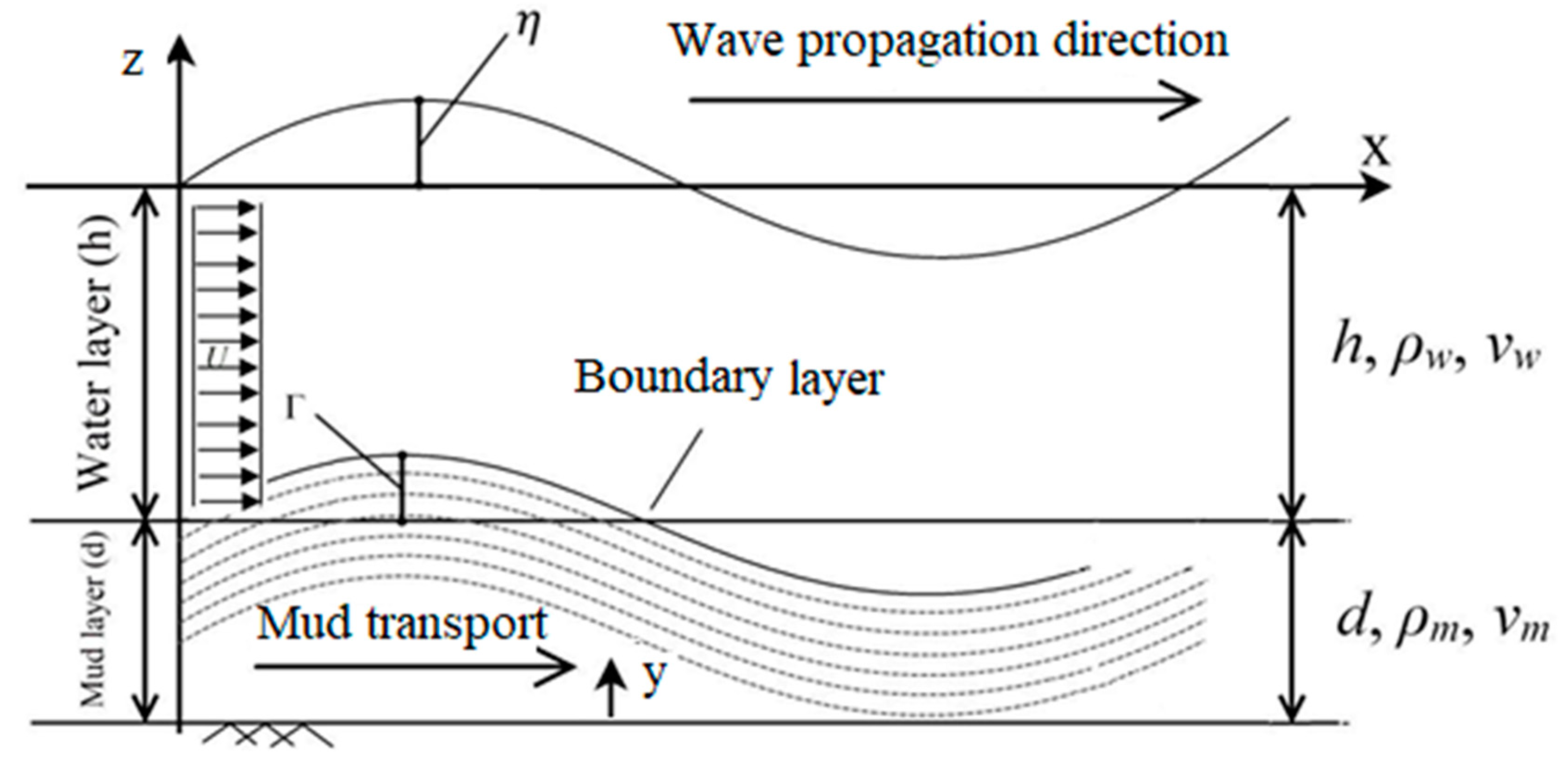
A two-layer model is considered in the present problem in which the upper layer is clear water, and the lower layer is liquid mud. A train of regular waves with wave number, k, and wave angular frequency, σ, and amplitude, a is traveling on a water surface overlying a fluid mud layer. In the model, ρ is the density, γ the dynamic viscosity, ν the viscosity, h the water depth, and d is the mud thickness. The subscripts w, m denote the water and mud respectively and, the free surface η and interface displacements Γ are shown in Figure 1.

2.1. Assumptions

The following assumptions have been made in analytical solutions:

• It is assumed that the current U is one dimensional, steady, and uniform (i.e., $\frac{\partial U}{\partial t}=0$, $\frac{\partial U}{\partial x}=0$),
• The mud layer is assumed as a Newtonian highly viscous fluid and, therefore, the current does not penetrate the mud layer. Because of such considerations, the solution is limited to the highly viscous/thin layers of mud,
• The current has been considered an order of magnitude larger than the wave-induced velocities,
• The wave amplitude, mud thickness, and the mud boundary layer thickness are assumed to be of the same orders and much smaller than the wave length. Thus, the water has been considered shallow, and the wave is long comparing to the mean water depth, and
• Spatial and temporal variation of mud properties is neglected.

2.2. Governing Equations

2.2.1. Water Layer

The governing Navier–Stokes equations in the water wave boundary layer, neglecting the fluctuating terms of convective accelerations (turbulent terms), and including one-dimensional current, are expressed as Equations (1)–(3) [1]. The boundary layer assumptions imply that $\frac{d^2}{d{x}^2}\ll \frac{d^2}{d{y}^2}$, and the vertical velocity components of the Navier–Stokes equations are neglected compared to the horizontal velocity. Therefore the pressure remains constant over the boundary layers (Equation (3)).

$$\frac{\partial \left({\tilde{u}}_w+U\right)}{\partial x}+\frac{\partial \left({\tilde{v}}_w\right)}{\partial y}=0$$

(1)

$$\begin{array}{r}\frac{\partial \left({\tilde{u}}_w+U\right)}{\partial t}+\left({\tilde{u}}_w+U\right)\frac{\partial \left({\tilde{u}}_w+U\right)}{\partial x}+\left({\tilde{v}}_w\right)\frac{\partial \left({\tilde{u}}_w+U\right)}{\partial y}\\ =-\frac{1}{{\rho }_w}\frac{\partial \left(P+{\tilde{p}}_w\right)}{\partial x}+{\nu }_w\frac{{\partial }^2\left({\tilde{u}}_w+U\right)}{\partial y^2}\end{array}$$

(2)

$$0=-\frac{1}{{\rho }_w}\frac{\partial \left(P+{\tilde{p}}_w\right)}{\partial y}$$

(3)

where $\left({\tilde{u}}_w,{\tilde{v}}_w\right)$ are the horizontal and vertical components of the fluctuating terms of water velocity, ${\tilde{p}}_w$ the dynamic fluctuating pressure in the water layer, $\left(x,y\right)$ the horizontal and vertical coordinates, t the time, $\left(U\right)$ the horizontal steady components of the water velocity (the vertical steady component is assumed zero, i.e., the current is one-dimensional), and $P$ is the averaged component of the dynamic pressure of water. It is assumed that the wave amplitude, mud thickness, and the mud boundary layer thickness are of the same orders and much smaller than the wave length, $ka~kd~k\delta \ll 1$, where $\delta$ is the boundary layer thickness. Thus, in the equations and the boundary conditions, the parameter $ϵ=ka$ has been inserted to indicate the relative asymptotic order of the associated term, based on the following scalings of the variables: x = O(k⁻¹), y = O(d), t = O(σ⁻¹), $\tilde{u}$ = O(σa), $\tilde{v}$= O($ϵ$σa), $\tilde{p}/\rho$= O(ga), $P/\rho =O\left(gh\right)$. The variables in the equations are expanded as: $L=L_1+\epsilon L_2+O\left({\epsilon }^2\right)$, where $L=\left(\tilde{u},\tilde{v},\tilde{p},P\right)$, and g is the gravitational acceleration.

Time averaging the Navier–Stokes equations (which is defined by $\overline{L}=\underset{T\to \infty }{\lim }\frac{1}{T}{{\displaystyle \int }}_0^T\widehat{L}dt$, for an arbitrary function $\widehat{L}$) in coexisting fluctuating and steady velocities gives the current equation:

$$\frac{\partial U}{\partial x}=0$$

(4)

$$ϵ\overline{{\tilde{u}}_w\frac{\partial {\tilde{u}}_w}{\partial x}}+ϵ\overline{{\tilde{v}}_w\frac{\partial {\tilde{u}}_w}{\partial y}}=-\frac{1}{{\rho }_w}\frac{\partial P}{\partial x}+{\nu }_w\frac{{\partial }^{2}U}{\partial y^2}+O\left({ϵ}^2\right)$$

(5)

$$0=-\frac{1}{{\rho }_w}\frac{\partial P}{\partial y}+O\left({ϵ}^2\right)$$

(6)

where the two terms on the left hand side of Equation (5) represent the effects of wave on the current field.

By subtracting current equations (Equations (4)–(6)) from the Navier–Stokes equations (Equations (1)–(3)) the wave equations are derived for the case of coexisting waves and currents.

$$\frac{\partial {\tilde{u}}_w}{\partial x}+\frac{\partial {\tilde{v}}_w}{\partial y}=0$$

(7)

$$\begin{array}{cc}\hfill \frac{\partial {\tilde{u}}_w}{\partial t}+ϵ{\tilde{u}}_w\frac{\partial {\tilde{u}}_w}{\partial x}& -ϵ\overline{{\tilde{u}}_w\frac{\partial {\tilde{u}}_w}{\partial x}}+ϵ{\tilde{v}}_w\frac{\partial {\tilde{u}}_w}{\partial y}-ϵ\overline{{\tilde{v}}_w\frac{\partial {\tilde{u}}_w}{\partial y}}+U\frac{\partial {\tilde{u}}_w}{\partial x}\hfill \\ & =-\frac{1}{{\rho }_w}\frac{\partial {\tilde{p}}_w}{\partial x}+{\nu }_w\frac{{\partial }^2{\tilde{u}}_w}{\partial y^2}+O\left({ϵ}^2\right)\hfill \end{array}$$

(8)

$$0=-\frac{1}{{\rho }_w}\frac{\partial {\tilde{p}}_w}{\partial y}+O\left({ϵ}^2\right)$$

(9)

where the sixth term at the left-hand side of the Equation (8) represents the effects of current on the wave field. On the other hand, the horizontal component of velocity in the inviscid flow near the water-mud interface is governed by:

$$\frac{\partial \left({\tilde{U}}_I+U\right)}{\partial x}=0$$

(10)

$$\frac{\partial \left({\tilde{U}}_I+U\right)}{\partial t}+ϵ\left({\tilde{U}}_I+U\right)\frac{\partial \left({\tilde{U}}_I+U\right)}{\partial x}=-\frac{1}{{\rho }_w}\frac{\partial \left(P+{\tilde{P}}_I\right)}{\partial x}+O\left({ϵ}^2\right)$$

(11)

where ${\tilde{U}}_I$, ${\tilde{P}}_I$ are the horizontal component of velocity and the dynamic pressure of the inviscid flow respectively. At a distance far from the boundary layer we have:

$$\left({\tilde{u}}_w,{\tilde{p}}_w\right)\to \left({\tilde{U}}_I,{\tilde{P}}_I\right)\hspace{1em}z=y-h-d\to -h$$

(12)

where z is the vertical coordinate measured from the water free surface.

2.2.2. Mud Layer

The governing Navier–Stokes equations in the mud layer are expressed as:

$$\frac{\partial {\widehat{u}}_m}{\partial x}+\frac{\partial {\widehat{v}}_m}{\partial y}=0$$

(13)

$$\frac{\partial {\widehat{u}}_m}{\partial t}+ϵ{\widehat{u}}_m\frac{\partial {\widehat{u}}_m}{\partial x}+ϵ{\widehat{v}}_m\frac{\partial {\widehat{u}}_m}{\partial y}=-\frac{1}{{\rho }_m}\frac{\partial {\widehat{p}}_m}{\partial x}+{\nu }_m\frac{{\partial }^2{\widehat{u}}_m}{\partial y^2}+O\left({ϵ}^2\right)$$

(14)

$$0=-\frac{1}{{\rho }_m}\frac{\partial {\widehat{p}}_m}{\partial y}+O\left({ϵ}^2\right)$$

(15)

where $\left({\widehat{u}}_m,{\widehat{v}}_m\right)$ represent the horizontal and vertical instantaneous components of the mud particles velocity, and ${\widehat{p}}_m$ is the dynamic pressure in the mud.

Time averaging Equations (13)–(15) gives the current equation in the mud layer;

$$ϵ\overline{{\tilde{u}}_m\frac{\partial {\tilde{u}}_m}{\partial x}}+ϵ\overline{{\tilde{v}}_m\frac{\partial {\tilde{u}}_m}{\partial y}}={\nu }_m\frac{{\partial }^2{U}_{Em}}{\partial y^2}+O\left({ϵ}^2\right)$$

(16)

$$0=-\frac{1}{{\rho }_m}\frac{\partial P_m}{\partial y}+O\left({ϵ}^2\right)$$

(17)

where $\left({\tilde{u}}_m,{\tilde{v}}_m\right)$ are the horizontal and vertical components of the fluctuating terms of mud velocity, P_m is the mean pressure, and $U_{Em}$ is the well-known Eulerian streaming velocity in the mud.

Similar to the water layer, by subtracting the Equations (16) and (17) from Equations (13)–(15), the wave equations in the mud layer are derived for the case of coexisting waves and currents.

$$\frac{\partial {\tilde{u}}_m}{\partial x}+\frac{\partial {\tilde{v}}_m}{\partial y}=0$$

(18)

$$\frac{\partial {\tilde{u}}_m}{\partial t}+ϵ{\tilde{u}}_m\frac{\partial {\tilde{u}}_m}{\partial x}-ϵ\overline{{\tilde{u}}_m\frac{\partial {\tilde{u}}_m}{\partial x}}+ϵ{\tilde{v}}_m\frac{\partial {\tilde{u}}_m}{\partial y}-ϵ\overline{{\tilde{v}}_m\frac{\partial {\tilde{u}}_m}{\partial y}}=-\frac{1}{{\rho }_m}\frac{\partial {\tilde{p}}_m}{\partial x}+{\nu }_m\frac{{\partial }^2{\tilde{u}}_m}{\partial y^2}+O\left({ϵ}^2\right)$$

(19)

$$0=-\frac{1}{{\rho }_m}\frac{\partial {\tilde{p}}_m}{\partial y}+O\left({ϵ}^2\right)$$

(20)

where ${\tilde{p}}_m$ is the fluctuating component of the dynamic pressure in the mud layer.

2.3. Physical Domain

In order to solve the governing equations to the first and second orders, the physical domain for each of the equations should be defined (Figure 1).

Table 1. Definition of the physical domains.

Sub-Domain	Definition Interval
Mud layer (M)	$0\le y\le d$
Water boundary layer (WB)	$d\le y<\infty$
Water core region (WC)	$0\le z<-h$

presents the domains of wave and current equations in water and mud layers.

Where $z=y-h-d$ is the vertical coordinate located on the water free surface and is necessary for the implementation of the free surface kinematic and dynamic boundary conditions (e.g., Equation (12)).

2.4. Boundary Conditions

The general kinematic and dynamic boundary conditions are defined at the domain and sub-domains boundaries (

Table 2. Definition of the boundary conditions.

No.	Boundary Conditions	Type	Domain
T1	${\widehat{u}}_m=0$	Kinematic	M
T2	${\widehat{u}}_m+ϵ\Gamma \frac{\partial {\widehat{u}}_m}{\partial y}={\widehat{u}}_w+ϵ\Gamma \frac{\partial {\widehat{u}}_w}{\partial y}$	Kinematic	M, WB
T3	${\widehat{v}}_m+ϵ\Gamma \frac{\partial {\widehat{v}}_m}{\partial y}={\widehat{v}}_w+ϵ\Gamma \frac{\partial {\widehat{v}}_w}{\partial y}$	Kinematic	M, WB
T4	${\rho }_w{\nu }_w\left(\frac{\partial {\widehat{u}}_w}{\partial y}+ϵ\Gamma \frac{{\partial }^2{\widehat{u}}_w}{\partial y^2}\right)={\rho }_m{\nu }_m\left(\frac{\partial {\widehat{u}}_m}{\partial y}+ϵ\Gamma \frac{{\partial }^2{\widehat{u}}_m}{\partial y^2}\right)$	Dynamic (shear stress)	M, WB
T5	${\widehat{P}}_w+ϵ\left(\Gamma \frac{\partial {\widehat{P}}_w}{\partial y}-{\rho }_w\mathrm{g}\Gamma \right)={\widehat{P}}_m+ϵ\left(\Gamma \frac{\partial {\widehat{P}}_m}{\partial y}-{\rho }_m\mathrm{g}\Gamma \right)$	Dynamic (normal stress)	M, WB
T6	$\frac{\partial \Gamma }{\partial t}+ϵ\widehat{u}\frac{\partial \Gamma }{\partial x}={\widehat{v}}_m$	Kinematic	M, WB
T7	$\frac{\partial \eta }{\partial t}+ϵ\widehat{u}\frac{\partial \Gamma }{\partial x}={\widehat{v}}_w$	Kinematic	WC
T8	${\widehat{P}}_w+ϵ\left(\Gamma \frac{\partial {\widehat{P}}_w}{\partial y}-{\rho }_w\mathrm{g}\Gamma \right)=0$	Dynamic (normal stress)	WC

).

Where $\Gamma =b{e}^{i\left(kx-\sigma t\right)}$, b is the amplitude of mud movement at the water-mud interface.

2.5. Solutions

2.5.1. First Order Solutions

Applying Equations (9), (12) and (20) and considering the continuity of normal stress at the water-mud interface (i.e., ${\tilde{p}}_{w1}={\tilde{p}}_{m1}$ in the first order), the leading order governing equations in water and mud layers are derived from Equations (18)–(20) as follows:

$$\frac{\partial {\tilde{u}}_{w1}}{\partial t}+U\frac{\partial {\tilde{u}}_{w1}}{\partial x}=\frac{\partial {\tilde{U}}_{I1}}{\partial t}+U\frac{\partial {\tilde{U}}_{I1}}{\partial x}+{\nu }_w\frac{{\partial }^2{\tilde{u}}_{w1}}{\partial y^2}$$

(21)

$$\frac{\partial {\tilde{u}}_{m1}}{\partial t}=\gamma \left(\frac{\partial {\tilde{U}}_{I1}}{\partial t}+U\frac{\partial {\tilde{U}}_{I1}}{\partial x}\right)+{\nu }_m\frac{{\partial }^2{\tilde{u}}_{m1}}{\partial y^2}$$

(22)

where $\gamma ={\rho }_m/{\rho }_w$ and subscript 1 denotes the first order solution.

Considering $\tilde{L}=L\left(y\right)e^{i\left(kx-\sigma t\right)}$ where $\tilde{L}={\tilde{u}}_{w1},{\tilde{u}}_{m1},{\tilde{U}}_{I1}$ the Equations (21) and (22) convert to the ordinary differential equations as follows:

$$\frac{d^2{u}_{w1}}{d{y}^2}+\frac{i\omega }{{\nu }_w}{u}_{w1}=\frac{i\omega }{{\nu }_w}{U}_{I1}$$

(23)

$$\frac{d^2{u}_{m1}}{d{y}^2}+\frac{i\sigma }{{\nu }_m}{u}_{m1}=\gamma \frac{i\omega }{{\nu }_m}{U}_{I1}$$

(24)

where $\omega =\sigma -Uk$ is the relative frequency.

The solution of the Equations (23) and (24) are written as follows:

$$u_{w1}=\left(1+E{e}^{-{\lambda }_w\left(y-d\right)}\right)U_{I1}$$

(25)

$$u_{m1}=\left[\frac{\omega }{\sigma }\gamma +Gcosh\left({\lambda }_{m}y\right)+Hsinh\left({\lambda }_{m}y\right)\right]U_{I1}$$

(26)

where ${\lambda }_f=\frac{1-\mathrm{i}}{{\delta }_f},$ in which f = w, m denotes water and mud respectively, and:

$${\delta }_w=\sqrt{\frac{2{\nu }_w}{\omega }},\hspace{1em}and\hspace{1em}{\delta }_m=\sqrt{\frac{2{\nu }_m}{\sigma }}$$

The leading order boundary conditions are the linearized form of boundary conditions in

Table 3. Wave and current conditions (h = 0.3 m, d = 0.11 m). “+” and “−” for the current velocity, U, refer to the following and opposing currents respectively.

T (s)	a (m)	νm (N/m2)	ρm (kg/m3)	U (m/s)
1.1	0.025	0.05~0.07	1345	−0.3~0.3

(T1–T3) and are written as $u_m=0$ at $y=0$; $u_m=u_w$ at $y=d$; and, ${\rho }_m{\nu }_m\frac{d{u}_m}{dy}={\rho }_w{\nu }_w\frac{d{u}_w}{dy}$ at $y=d$, thus, the constant coefficients of Equations (25) and (26) are obtained as follows:

$$G=-\frac{\omega }{\sigma }\gamma ,$$

$$E=\frac{\left\{\frac{\omega }{\sigma }\gamma \left[{\zeta }^2\xi sinh\left({\lambda }_{m}d\right)+\gamma cosh\left({\lambda }_{m}d\right)\right]+\gamma \right\}sinh\left({\lambda }_{m}d\right)}{sinh\left({\lambda }_{m}d\right)+{\zeta }^2\xi cosh\left({\lambda }_{m}d\right)}+\frac{\omega }{\sigma }\gamma \left(1-cosh\left({\lambda }_{m}d\right)\right)-1,$$

$$H=\frac{\frac{\omega }{\sigma }\gamma \left({\zeta }^2\xi sinh\left({\lambda }_{m}d\right)+\gamma cosh\left({\lambda }_{m}d\right)\right)+\gamma }{sinh\left({\lambda }_{m}d\right)+{\zeta }^2\xi cosh\left({\lambda }_{m}d\right)}$$

where, $\xi =\frac{{\lambda }_m}{{\lambda }_w}$, $\zeta ={\left(\frac{{\nu }_m}{{\nu }_w}\right)}^{1/2}$.

The vertical component of the velocity, on the other hand, is obtained by integration of the horizontal velocity

$$v_{m1,w1}\left(y\right)=-ik{{\displaystyle \int }}_0^y{u}_{m1,w1}\left(y\right)dy$$

(27)

$$v_{m1}\left(y\right)=-ik\left[\frac{\omega }{\sigma }\gamma y+G_1\sinh \left({\lambda }_{m}y\right)+H_1\left(\cosh \left({\lambda }_{m}y\right)-1\right)\right]U_{I1}$$

(28)

$$v_{w1}\left(y\right)=v_{m1}\left(d\right)-ik\left[y-d-E_1\left(e^{-{\lambda }_w\left(y-d\right)}-1\right)\right]U_{I1}$$

(29)

where,

$$G_1,H_1=\left(G,H\right)/{\lambda }_m,\hspace{1em}{E}_1=E/{\lambda }_w$$

$$G_2,H_2=\left(G,H\right){\lambda }_m,\hspace{1em}{E}_2=E{\lambda }_w$$

The general solution of the linearized Navier–Stokes equations in the water layer including a uniform steady current which is valid both near and far from boundary layers is obtained as [10]:

$$u_w=A_w\cosh k\left(h+z\right)+B_w\sinh k\left(h+z\right)+D_w{e}^{-{\lambda }_w\left(h+z\right)}$$

(30)

$$v_w=-i\left(A_w\sinh k\left(h+z\right)+B_w\cosh k\left(h+z\right)-\frac{k{D}_w}{{\lambda }_w}{e}^{-{\lambda }_w\left(h+z\right)}\right)$$

(31)

The five unknowns of, $A_w$, $B_w$, $D_w$, k, and U_I1 are obtained from the following boundary conditions (Equations (32) and (34)–(36)), which are relevant to the linearized form of the boundary conditions, T3, T7, and T8 in Table 2, and asymptotic conditions (Equation (33)):

$$u_{wc}=U_{I1},\hspace{1em}z\to -h$$

(32)

$$u_w=\left(1+E{e}^{-{\lambda }_w\left(y-d\right)}\right)U_{I1},\hspace{1em}z\to -h\hspace{1em}$$

(33)

$$v_w=v_{m1}\left(d\right),\hspace{1em}z\to -h$$

(34)

$$\frac{\partial \eta }{\partial t}+U\frac{\partial \eta }{\partial x}=v_w,\hspace{1em}z=0$$

(35)

$$\frac{\partial u_w}{\partial t}=-g\frac{\partial \eta }{\partial x},\hspace{1em}z=0$$

(36)

where $u_{wc}$ is the inviscid core solution containing the first two terms of Equations (30) and (31).

By applying the above linearized kinematic free surface boundary conditions and matching the asymptotic limit of vertical velocity (Equation (34)), the unknowns are found in terms of the wave number, k, as follows:

$$A_w=U_{I1},\hspace{1em}{D}_w=E_1{U}_{I1}$$

$$U_{I1}=\frac{\omega a}{\left(\sinh \left(kh\right)+B\cosh \left(kh\right)\right)}$$

(37)

$$B=k\left(\frac{\omega }{\sigma }\gamma d+G_1\sinh \left({\lambda }_{m}d\right)+H_1\left(\cosh \left({\lambda }_{m}d\right)-1\right)+E_1\right)$$

(38)

where $\omega$ represents the effect of current in Equations (37) and (38).

The dispersion relation including the effect of current is expressed as:

$$\frac{\sigma \left(\sigma -Uk\right)}{gk}=\frac{B+\tanh kh}{1+B\tanh kh}$$

(39)

The dissipation rate is the imaginary part of the dispersion relation (39).

The amplitude of the mud movements is obtained as:

$$b=\left(k/\omega \right)\left[\frac{\omega }{\sigma }\gamma d+G_{1}sinh\left({\lambda }_{m}d\right)+H_1\left(cosh\left({\lambda }_{m}d\right)-1\right)\right]U_{I1}$$

(40)

The phase shift between the mud and water layer is written as:

$$\phi =\arctan \left(b_i/b_r\right)$$

(41)

2.5.2. Second Order Solutions

Since the steady current velocity should be a real value, considering Equation (19), and by identity, it can be shown that:

$${\nu }_m\frac{d^2{U}_{Em}}{d{y}^2}=\overline{\mathrm{Re}\left(v_{m1}{e}^{i\left(kx-\sigma t\right)}\right)\mathrm{Re}\left(\frac{d{u}_{m1}}{dy}{e}^{i\left(kx-\sigma t\right)}\right)}=\left(1/2\right)\mathrm{Re}\left(v_{m1}{\frac{d{u}_{m1}}{dy}}^{\ast }\right)$$

(42)

where * denotes the complex conjugate. Substitution of the real and imaginary parts of, $v_{m1}$,${\frac{d{u}_{m1}}{dy}}^{\ast }$ and twice integration, we will have the Eulerian streaming velocity in the mud layer (for further details, see Appendix A):

$$\begin{array}{cc}\hfill {\nu }_m{U}_{Em}& =\left(\frac{1}{2}k{\left|U_I\right|}^2\right)(I_{ch}\cosh \left(2{\lambda }_{mr}y\right)+I_c\cos \left(2{\lambda }_{mi}y\right)+I_s\sin \left(2{\lambda }_{mi}y\right)\hfill \\ & +I_{sh}\sinh \left(2{\lambda }_{mr}y\right)\hfill \\ & +P_{ss}\sinh \left({\lambda }_{mr}y\right)\sin \left({\lambda }_{mi}y\right)+P_{cc}\cosh \left({\lambda }_{mr}y\right)\cos \left({\lambda }_{mi}y\right)\hfill \\ & +P_{sc}\sinh \left({\lambda }_{mr}y\right)\cos \left({\lambda }_{mi}y\right)+P_{cs}\cosh \left({\lambda }_{mr}y\right)\sin \left({\lambda }_{mi}y\right)\hfill \\ & +P_{ycs}\frac{2{\lambda }_{mr}{\lambda }_{mi}}{{\left|{\lambda }_m\right|}^4}y+M_{1}y+M_2\hfill \end{array}$$

(43)

where,

$$I_{ch}=\frac{I}{8{\lambda }_{mr}{}^2},I_c=\frac{I\prime }{8{\lambda }_{mr}{}^2},\hspace{1em}{I}_s=\frac{II}{8{\lambda }_{mr}{}^2},\hspace{1em}{I}_{sh}=\frac{III}{8{\lambda }_{mr}{}^2},$$

and, I, I′, II, III, $P_{ycs}$, $P_{ss}$, $P_{cc}$, $P_{sc}$, $P_{cs}$ are defined in Appendix A, and M₁ and M₂ are constants obtained from the boundary conditions.

Similar to the mud layer, the governing equations for the Eulerian streaming velocity in the water boundary layer is written as follows:

$${\nu }_w\frac{d^2{U}_{Ew}}{d{y}^2}=\left(1/2\right)\mathrm{Re}\left(v_{w1}{\frac{d{u}_{w1}}{dy}}^c\right)$$

(44)

By substitution of the real and imaginary parts and twice integration, we will have the Eulerian streaming velocity in the water layer (the details have been provided in Appendix A) as:

$$\begin{array}{cc}\hfill {\nu }_w{U}_{Ew}& =\left(\frac{1}{2}k{\left|U_I\right|}^2\right)(I_{UEw}{e}^{-2{\lambda }_{wr}\left(Y\right)}+I{I}_{UEw}{e}^{-{\lambda }_{wr}\left(Y\right)}\left(\sin \left({\lambda }_{wi}Y\right)+\cos \left({\lambda }_{wi}Y\right)\right)\hfill \\ & +II{I}_{UEw}{e}^{-{\lambda }_{wr}\left(Y\right)}\left(\sin \left({\lambda }_{wi}Y\right)-\cos \left({\lambda }_{wi}Y\right)\right)+\hfill \\ & +E_{2i}\left(\frac{-{\lambda }_{wr}}{{\left|{\lambda }_w\right|}^2}Y{e}^{-{\lambda }_{wr}\left(Y\right)}\left(\sin \left({\lambda }_{wi}Y\right)+\cos \left({\lambda }_{wi}Y\right)\right)+\frac{2{\lambda }_{wr}{\lambda }_{wi}}{{\left|{\lambda }_w\right|}^4}{e}^{-{\lambda }_{wr}\left(Y\right)}\sin \left({\lambda }_{wi}Y\right)\right)\hfill \\ & -E_{r2}(\frac{-{\lambda }_{wr}}{{\left|{\lambda }_w\right|}^2}Y{e}^{-{\lambda }_{wr}\left(Y\right)}\left(\sin \left({\lambda }_{wi}Y\right)-\cos \left({\lambda }_{wi}Y\right)\right)\hfill \\ & -\frac{2{\lambda }_{wr}{\lambda }_{wi}}{{\left|{\lambda }_w\right|}^4}{e}^{-{\lambda }_{wr}\left(Y\right)}\cos \left({\lambda }_{wi}Y\right))+W_{1}y+W_2\hfill \end{array}$$

(45)

where

$$I_{UEw}=\frac{-I_w}{2{\lambda }_{wr}},\hspace{1em}I{I}_{UEw}=-I{I}_w\frac{{\lambda }_{wr}}{{\left|{\lambda }_w\right|}^2},\hspace{1em}II{I}_{UEw}=-II{I}_w\frac{{\lambda }_{wr}}{{\left|{\lambda }_w\right|}^2}$$

where $\left|{\lambda }_w\right|=\sqrt{{\lambda }_{wr}{}^2+{\lambda }_{wi}{}^2}$, and, $Y=y-d$, indexes i and r represent the imaginary and real parts respectively (the details are provided in Appendix A).

The following boundary conditions are the second-order boundary conditions and derived from the boundary conditions shown in Table 2.

$$U_{Em}=0;\hspace{1em}y=0$$

(46)

$$U_{Em}+\overline{\Gamma \frac{\partial u_{m1}}{\partial y}}=U_{Ew}+\overline{\Gamma \frac{\partial u_{w1}}{\partial y}};\hspace{1em}y=d$$

(47)

$${\rho }_m{\nu }_m\left(\frac{d{U}_{Em}}{dy}+\overline{\Gamma \frac{{\partial }^2{u}_{m1}}{\partial y^2}}\right)={\rho }_w{\nu }_w\left(\frac{d{U}_{Ew}}{dy}+\overline{\Gamma \frac{{\partial }^2{u}_{w1}}{\partial y^2}}\right)\hspace{1em}y=d$$

(48)

$$\frac{d{U}_{Ew}}{dy}\to 0;\hspace{1em}y\to \infty$$

(49)

The Equations (46) and (47) are kinematic conditions (non-slip condition and continuity of the velocities respectively), while the Equation (48) demonstrates the continuity of the second-order mean shear stress, and Equation (49) implies that the mean wave-induced second-order shear stress approaches zero outside the wave boundary layer. Applying the above boundary layer conditions W₁, W₂, M₁, and M₂ are obtained,

$$M_2=\left(\frac{1}{2}k{\left|U_I\right|}^2\right)\left(-P_{cc}-I_{ch}-I_c\right),\hspace{1em}{W}_1=0_{}$$

and, M₁, W₂, is obtained as described in Appendix B.

The mass transport velocity is the sum of Eulerian streaming velocity, and Stokes drift velocity [36]

$$U_{MTM}=U_{Em}+U_{sm}$$

(50)

$$U_{sm}=\overline{{\displaystyle \int }{u}_{m1}dt\frac{\partial u_{m1}}{\partial x}}+\overline{{\displaystyle \int }{v}_{m1}dt\frac{\partial u_{m1}}{\partial y}}$$

(51)

where $U_{sm}$ is the Stokes drift, and $U_{MTM}$ is the mass transport velocity both in the mud layer. The Stokes drift is defined as:

$$U_{sm}=\left(\frac{1}{2}k/\sigma {\left|U_I\right|}^2\right)\left(u_{mr}{}^2+u_{mi}{}^2-v_{mmr}{\frac{d{u}_m}{dy}}_r-v_{mmi}{\frac{d{u}_m}{dy}}_i\right)$$

(52)

where $v_{mm}=i{v}_m$, and the details have been presented in Appendix B.

3. Results and Discussion

3.1. Analytical Results

The wave and current conditions were selected in the ranges of experimental conditions of Soltanpour et al. [10] (Table 3). The wave amplitude is of the same order as the mud boundary layer thickness.

3.1.1. Particle Velocity

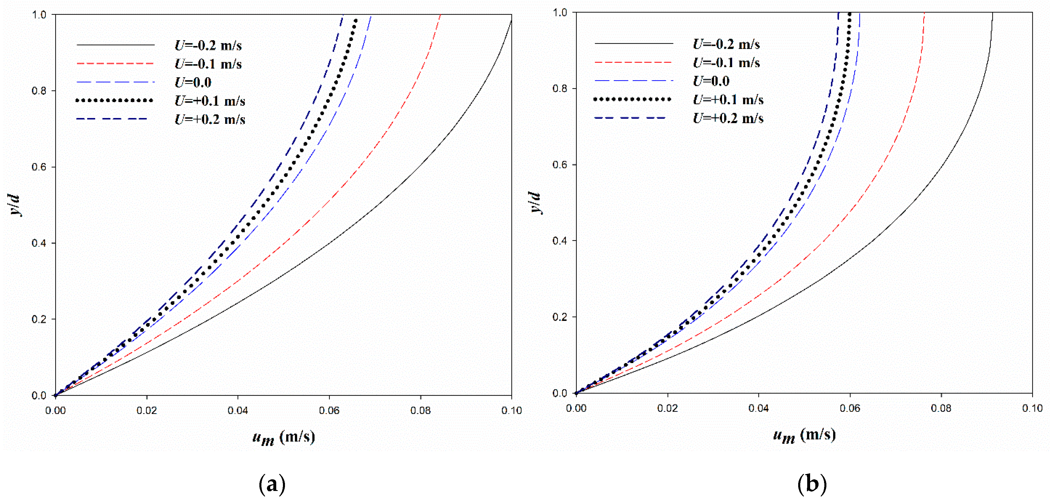
Profiles of mud maximum particle velocity for two different values of ζ show that the velocity profile approaches a vertical slope at the mud interface (i.e., providing zero shears) in the case of smaller viscosities (e.g., higher values of ζ, Figure 2). However, a fully shear layer is formed in the case of lower values of ζ (Figure 2). Besides, it is seen in the figure that the following current provides lower values of particle velocities compared to the no current and opposing current cases. The first term at the right-hand side of Equation (26) represents the effect of current on mud particle velocities.

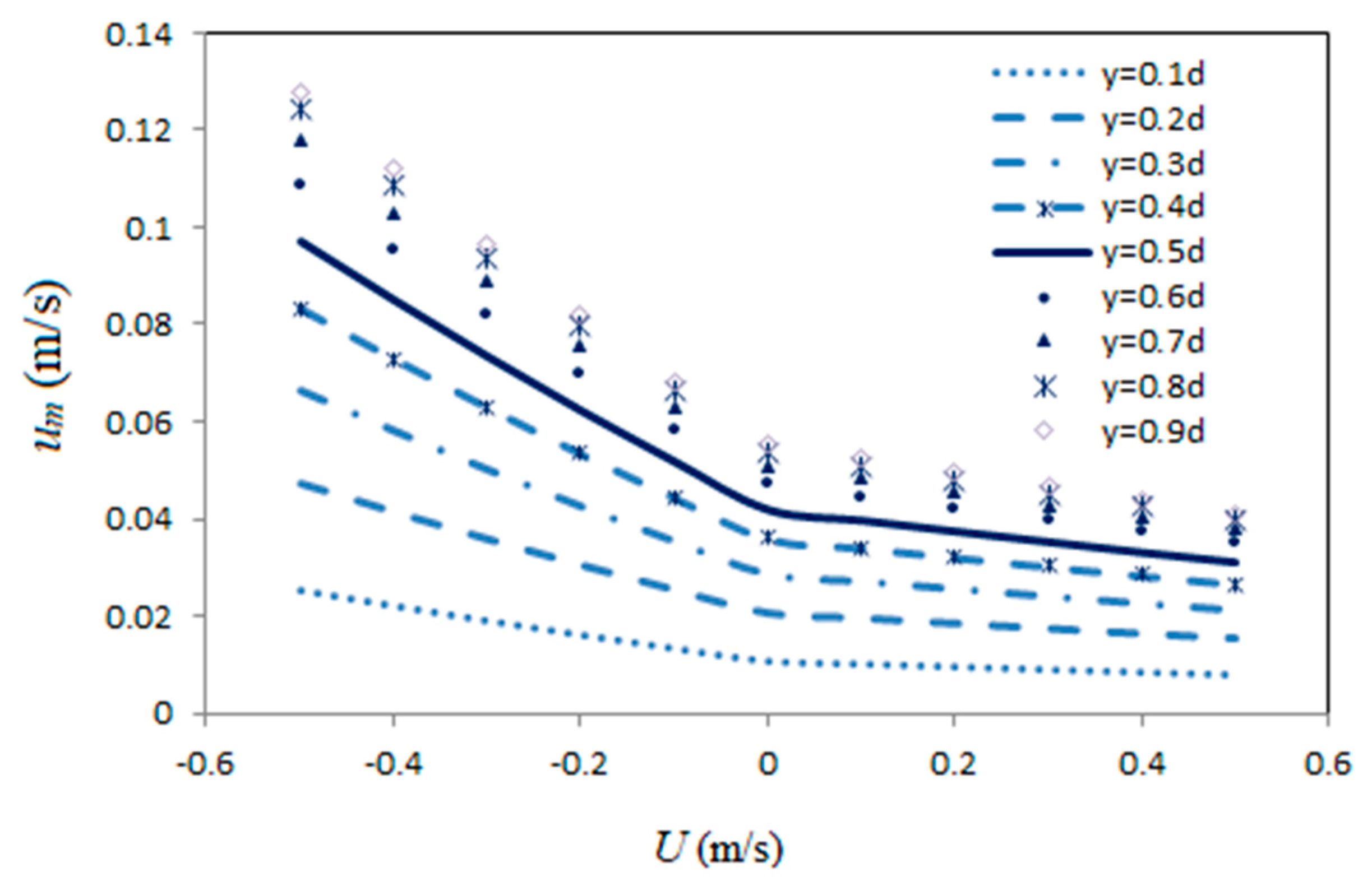
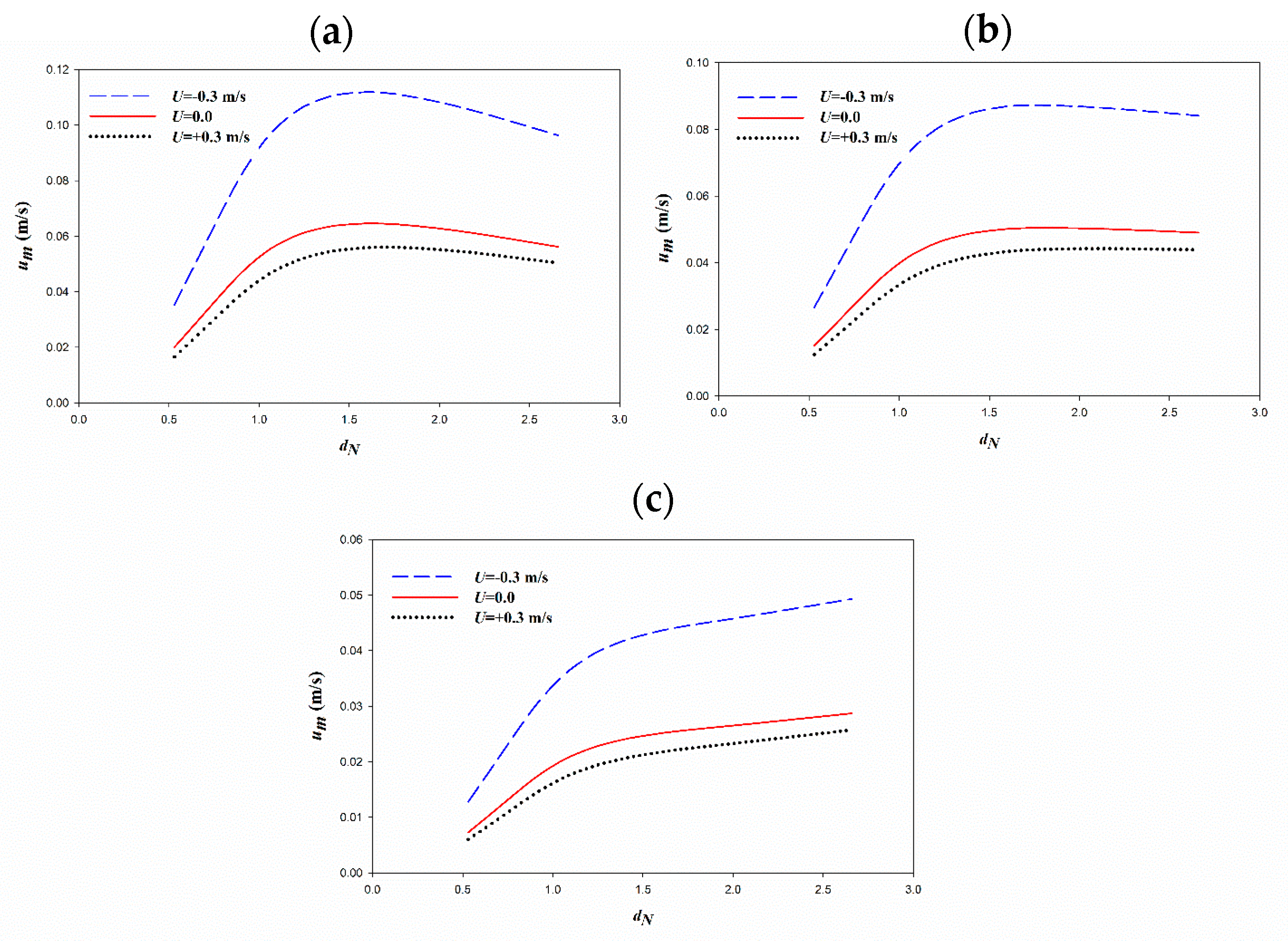
As discussed in Figure 2, by an increase in the current velocity, the particle velocity amplitudes are decreased (confirmed by Figure 3). This is because, by an increase in the current velocity, the wave length is increased, which results in a decrease in the mud movements. In addition, it is observed in the Equation (26), that by an increase in the current velocity, the relative frequency, ω is decreased, which results in the decrease of particle velocity (the first term at the right-hand side of Equation (26)). A similar trend was reported by An and Shibayama [26], with the same slope in the opposing and following currents. Particle velocity amplitudes versus dimensionless mud thickness are comparable with the results of dissipation rates (versus dimensionless mud thickness) provided by Ng [15] (Figure 4). As can be seen in the figure, the particle velocity values increase by an increase in the dimensionless mud thickness and then decrease. There is a local peak in dimensionless mud thickness around d_N = 1.2. The local peak is comparable to the model outputs for the dissipation rates of regular water waves versus the dimensionless mud thicknesses (e.g., [11,15]). By going deeper into the mud layer, the decrement phase is not obvious (e.g., the velocity amplitude remains constant or becomes ascending, corresponding to Figure 4b,c). This is relevant to the fact that deeper parts of the mud layer experience lower interactions with the water layer compared to the shallower parts and also to the fact that the current velocity is an order of magnitude larger than the wave-induced velocity (i.e., $U\gg \left|\tilde{u}\right|$).

3.1.2. Dissipation Rates

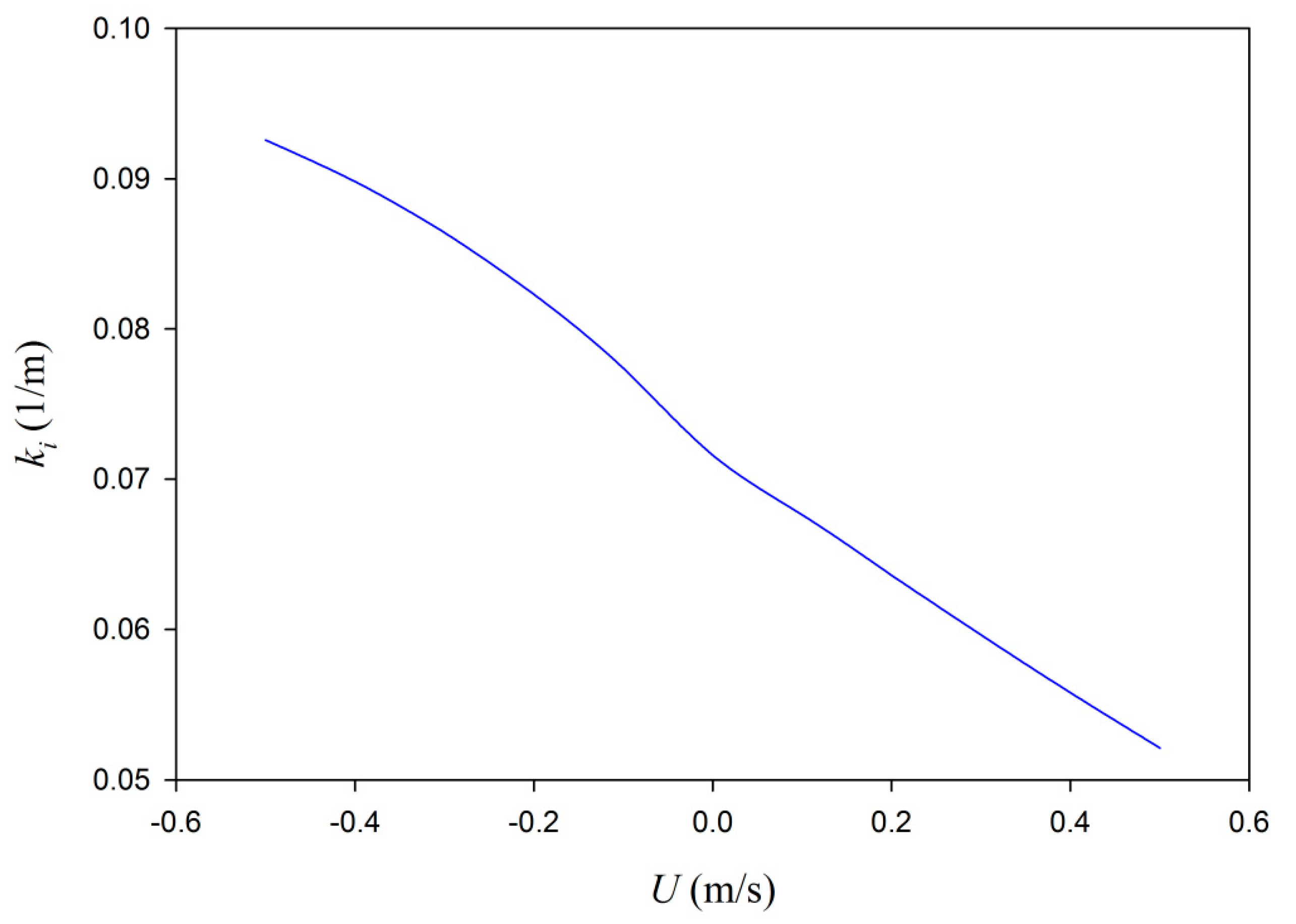
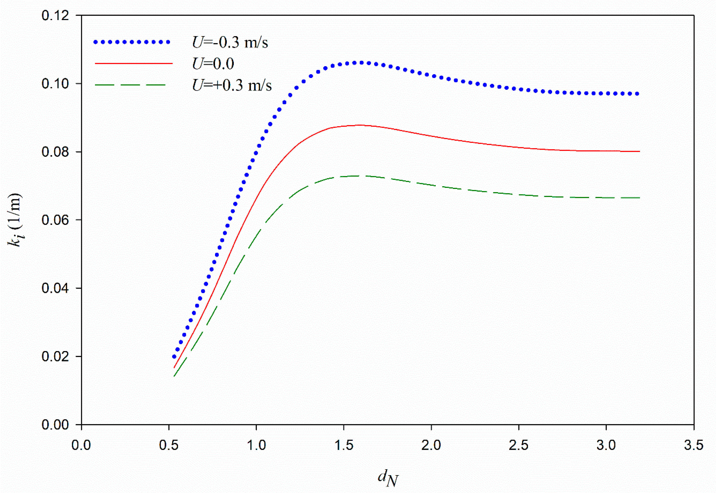
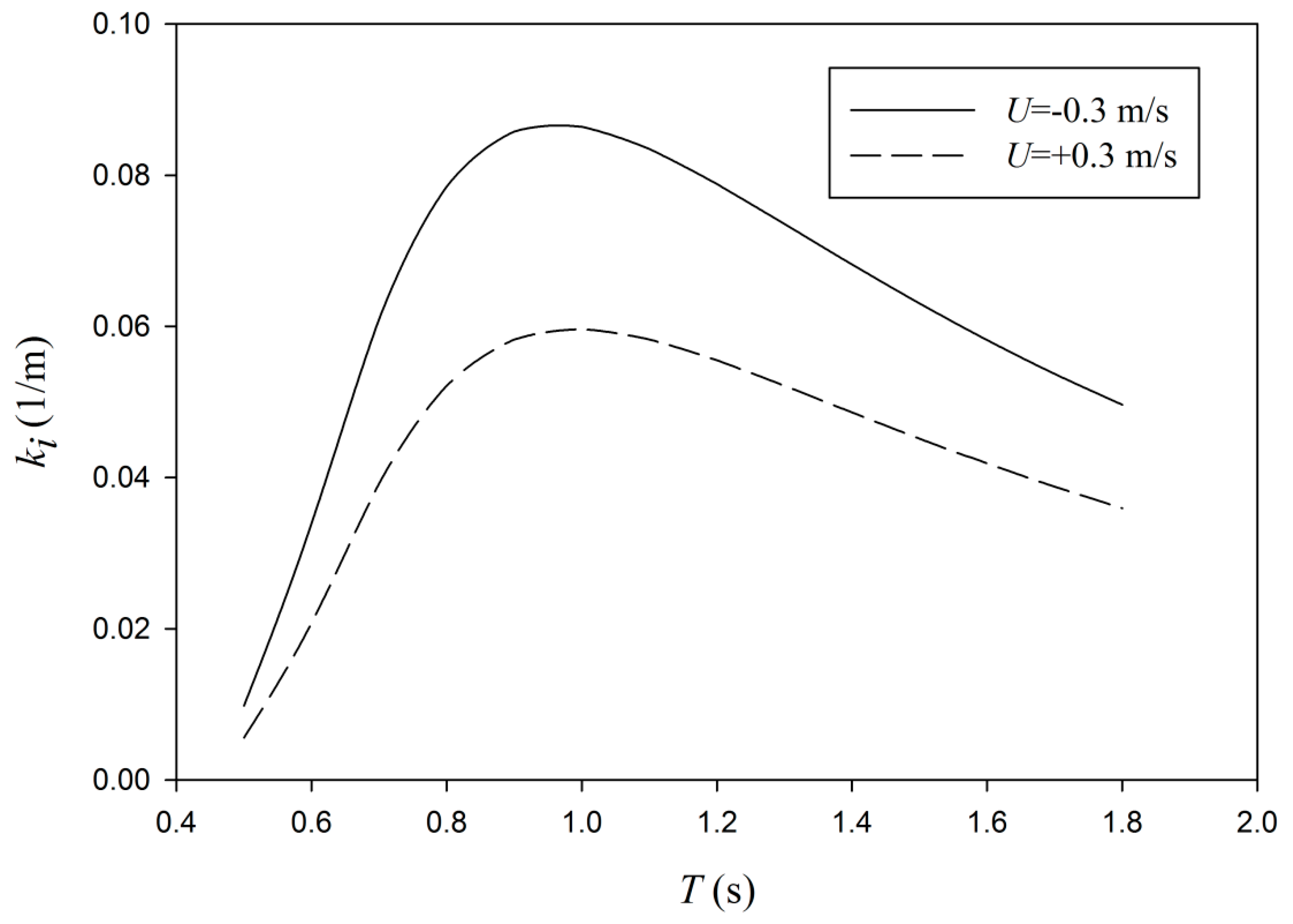
The variations of dissipation rates versus current velocity confirm the conclusions from Figure 3 that by a shift from negative to positive values of current velocity (i.e., opposing current to the following current), the dissipation rates decrease (Figure 5). This is because opposing current results in the smaller values of wavelengths, while the following current makes bigger wave lengths. Therefore, the wave number induced by the opposing current increases, and a higher wave attenuation rate is observed [10]. It is also directly observed from Equation (39) that the dissipation rate is a function of coefficient B and since the coefficient B is a function of relative frequency, ω (the first term at the right-hand side of Equation (38)), by an increase in the current velocity, the dissipation rate is decreased, which was not presented in previous analytical models. Dissipation rates versus dimensionless mud thickness, d_N shows a local peak (Figure 6), which is the comparable to the local peak presented by the viscous models (e.g., [11,12,15,23]) with the difference in the inclusion of current effects in the equations and results. The local peak also exists for the dissipation rates versus the wave period (Figure 7). The viscous models predict one local peak for the variations of wave dissipation rates versus the period and dimensionless mud thickness (e.g., [11,25]). Although the current does not change the trends, the values of the dissipation rates are affected by the currents (Figure 6 and Figure 7).

3.1.3. Phase Shift

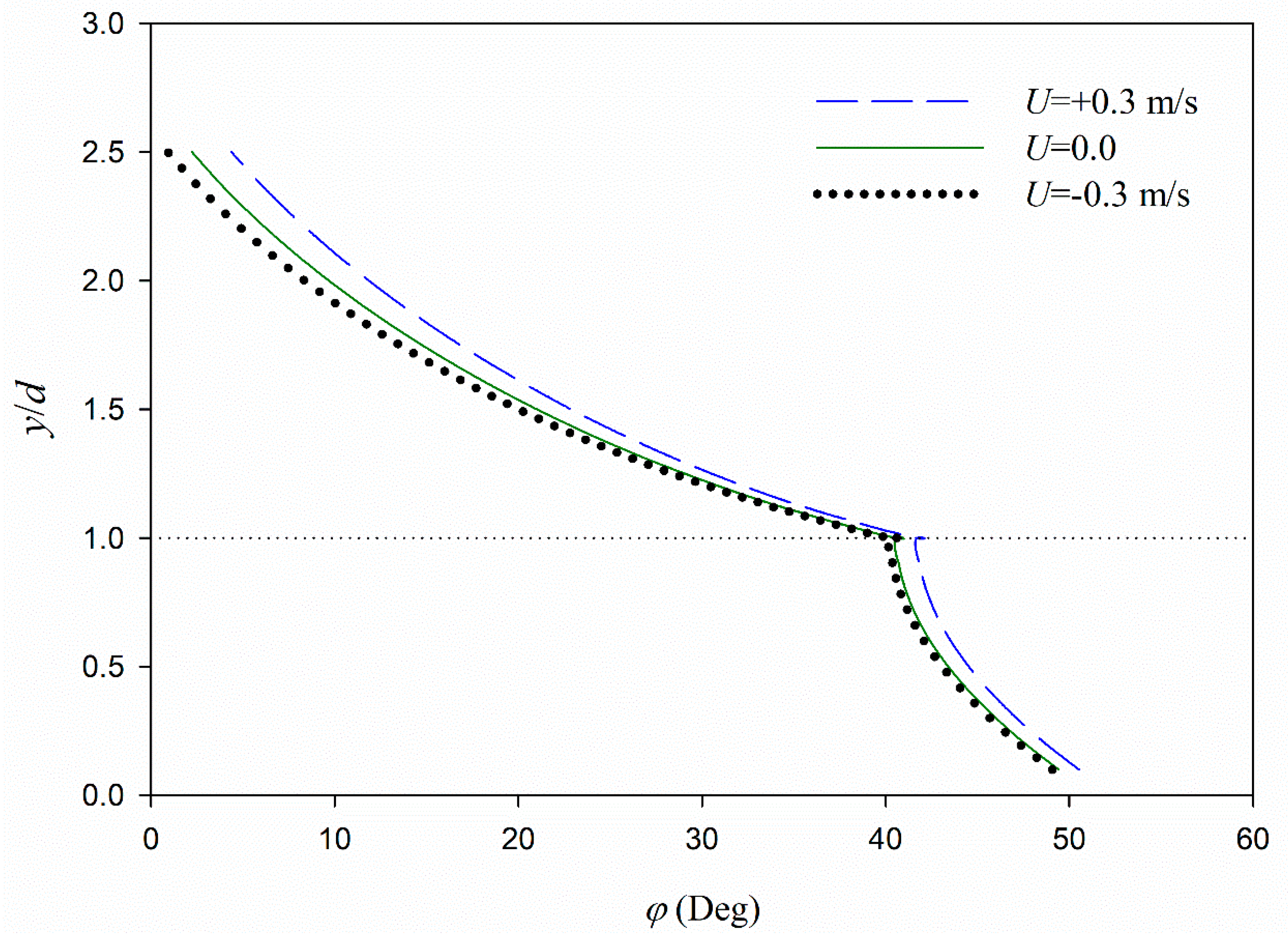
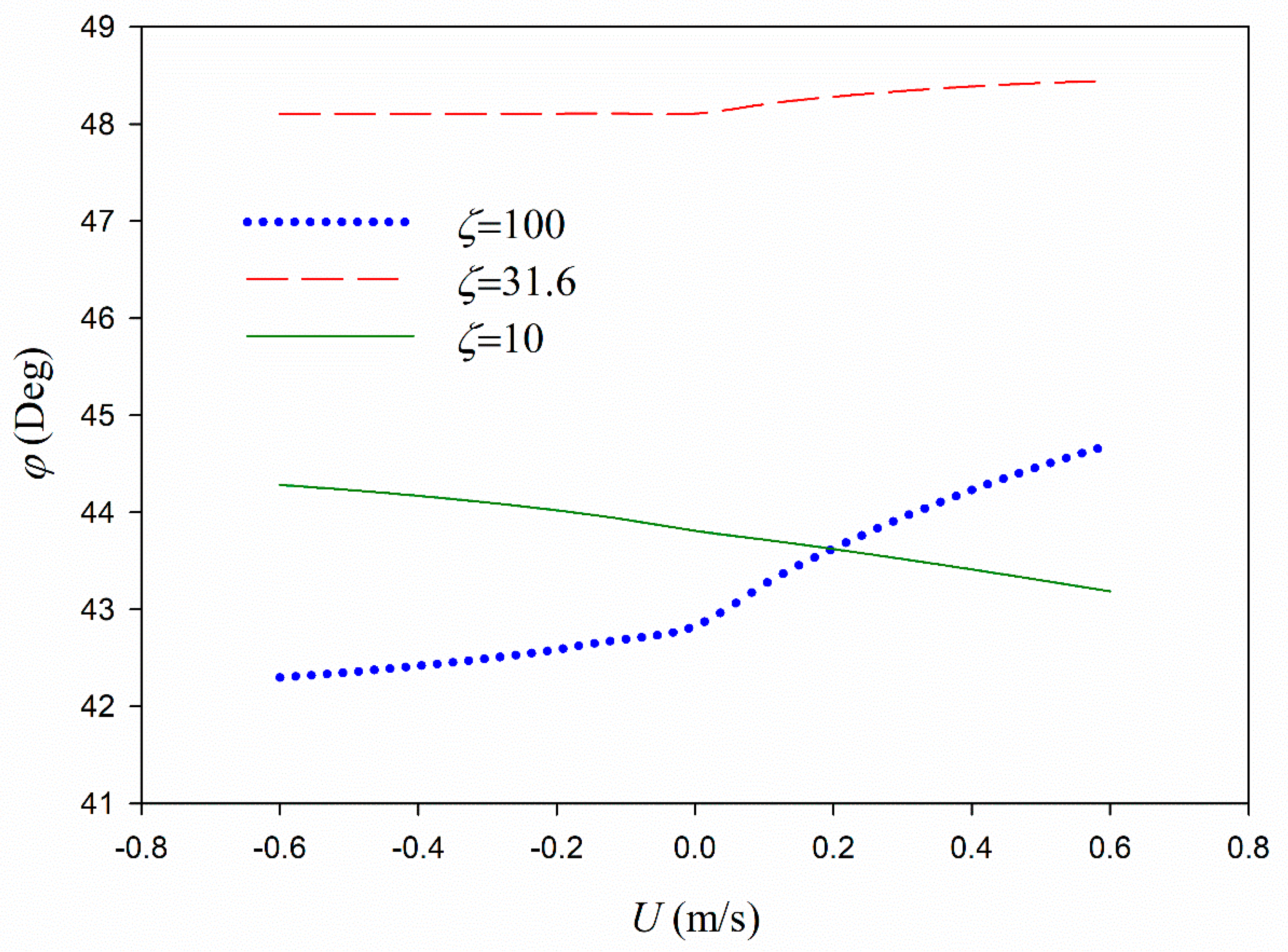
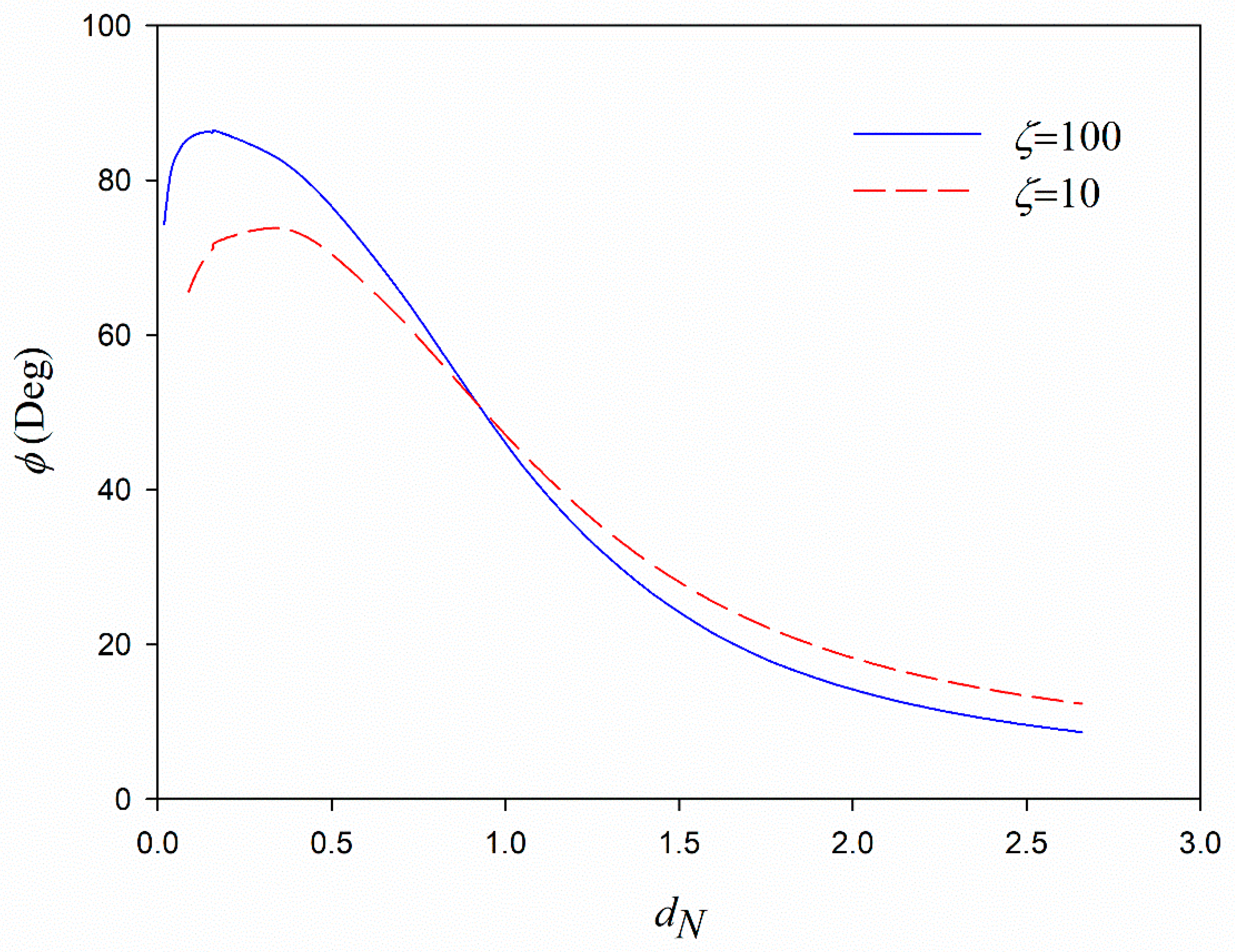
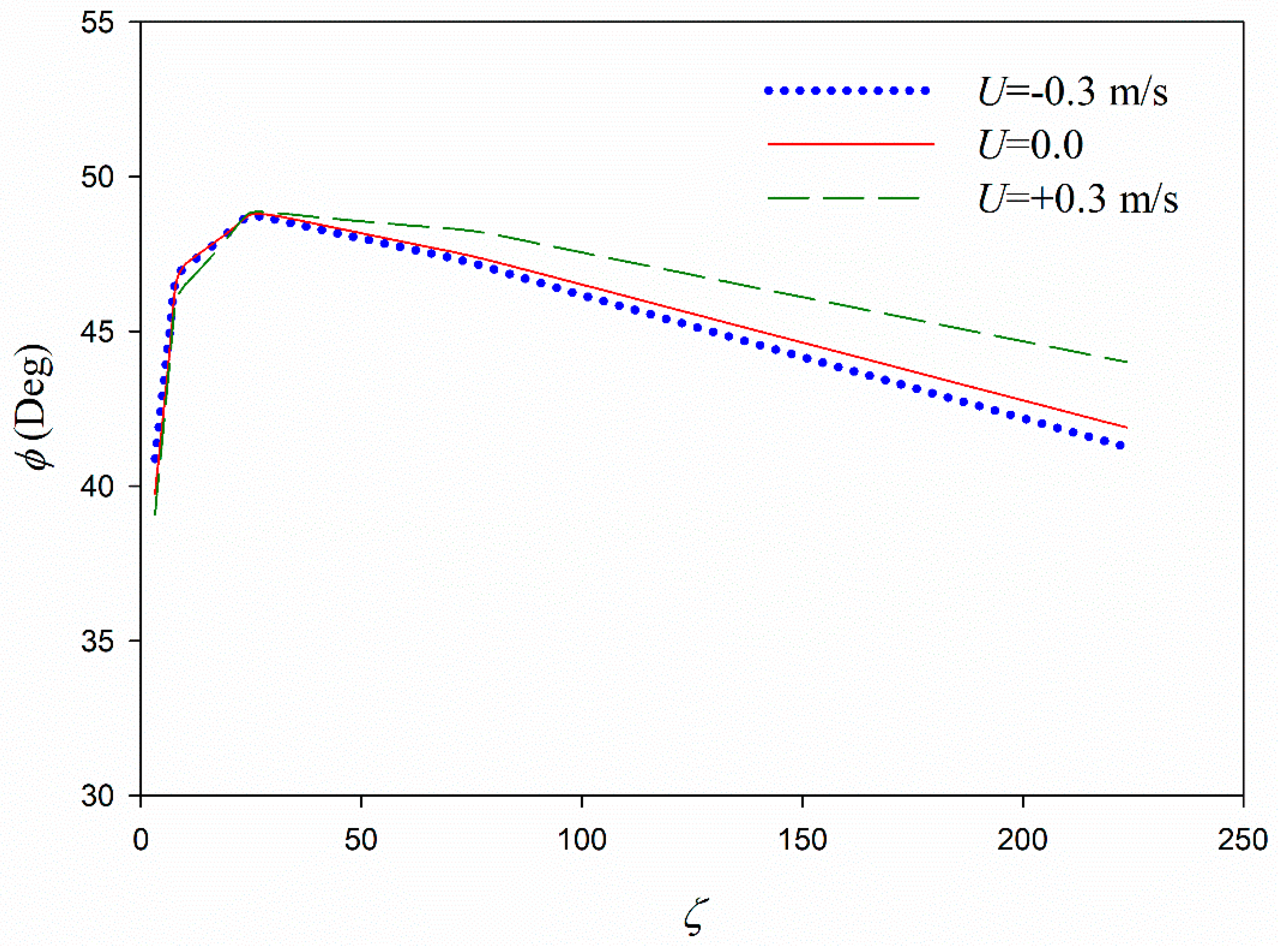
The phase shift decreases by going up from the mud layer into the water layer (Figure 8). The values of phase shift in the mud layer are in the category (45–65 Deg.) provided by Maa and Mehta [37]. The phase shift in the water is caused by the mud existence and the water boundary layer [10]. It is shown in Figure 8 that the phase shift is lower in the opposing current, while higher in the following current. However, the phase shift is highly dependent upon the mud/water viscosity ratio and a clear trend for the phase shift versus the current velocity is only observed at certain ranges of viscosities (Figure 9). Similar to the dissipation rates, the phase shift experiences a local peak over the dimensionless mud thickness (Figure 10). It is also confirmed that the effects of current on the phase shift depend on the values of the viscosity ratios (Figure 11).

3.1.4. Mud Mass Transport

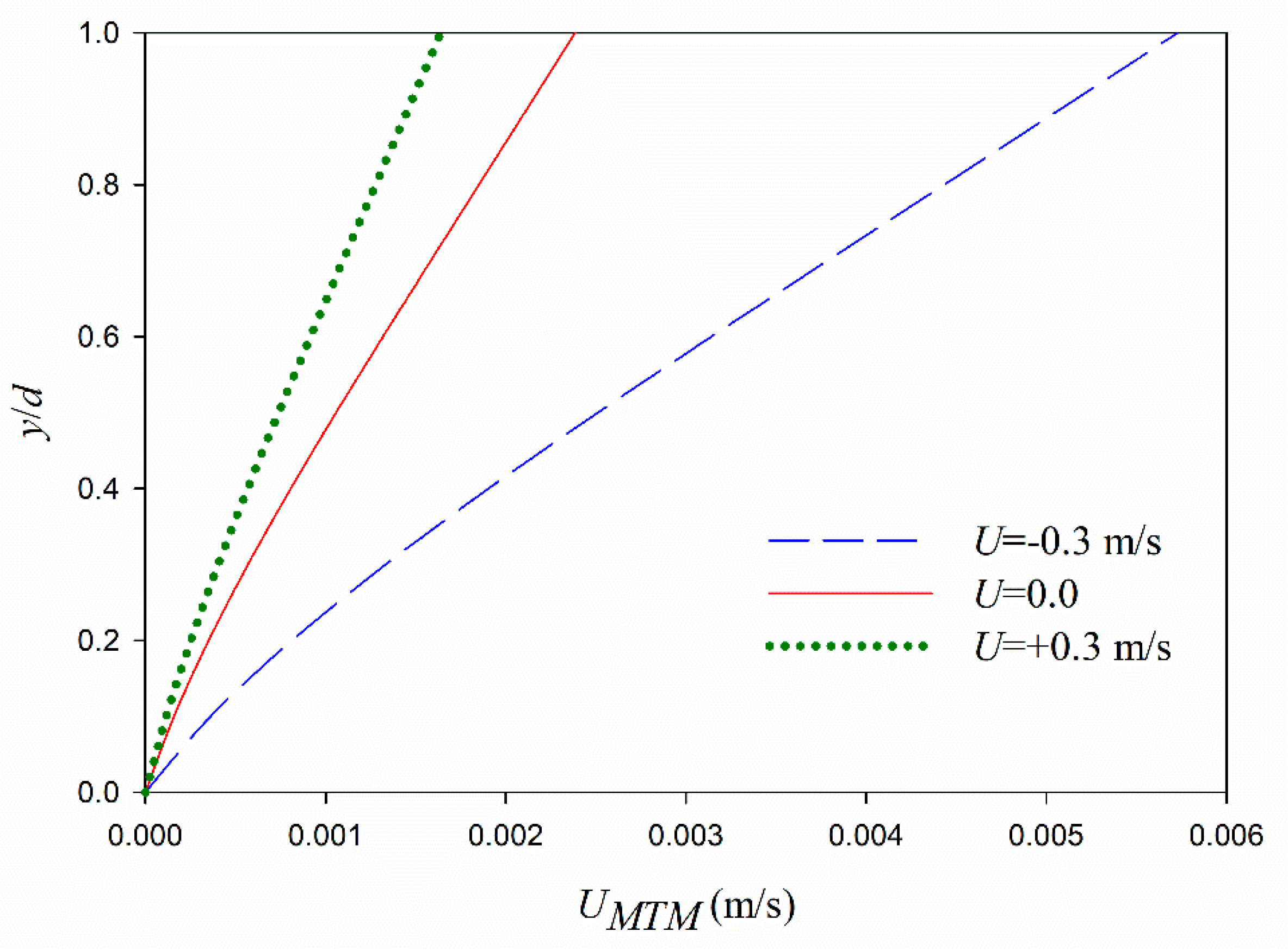
The profiles of the mud mass transport velocity for three representative following, opposing, and no current cases include the effects of current for the first time (Figure 12). As can be seen, the mass transport velocity is increased by a shift from the following current to the opposing current. The mud mass transport rates are increased by an increase in the mud dimensionless thickness (Figure 13). Besides, by shifting from the following current to the opposing current, the mass transport rates increase. As mentioned above (Figure 3 and Figure 4), the current has directly affected the mud mass transport, which is because the current velocity is larger than the wave-induced velocities.

3.2. Comparison with the Laboratory Data

3.2.1. First Test Case

In this section, the results of laboratory experiments carried by Soltanpour et al. [10] have been used for the verification of the proposed analytical model. A mixture of kaolinite and tap water was used as the fluid mud layer with a thickness of 0.11 m. The flume was then slowly filled with tap water, up to the total depth of 0.4 m, to avoid disturbing the mud layer (Figure 14).

The electromagnetic current meter (ECM, VM-801H, KENEC, Tokyo, Japan), proved to be applicable in both the clear water and highly concentrated fluid mud (400 kg/m³), was adopted in the measurements of Soltanpour et al. [10]. ECMs were fixed at the preselected locations above the bed (y = 0.02, 0.05, 0.085 m above the rigid bottom) to capture the particle velocities in the fluid mud layer [10]. The accuracy of the devices in the measuring ranges of 0–25 cm/s is ±2% [10]. Different wave characteristics and current values were considered in the laboratory tests (

Table 4. Laboratory experiments conditions.

No.	T (s)	a (m)	Water Content Ratio (%)	U (m/s)
1	1.0	0.0488	160	0.0471
2	1.1	0.03465	160	0
3	1.2	0.021	160	−0.1075
4	1.2	0.02	160	0.07
5	1.2	0.02	160	0
6	1.2	0.02	160	−0.1
7	1.1	0.0233	160	0.0985

). The ranges of wave periods and heights can well represent the real field conditions during the calm weather. The small amplitude of the wave heights (O (2 cm)) that is of the same order as the mud thickness (O (10 cm)) and the mud boundary layer thickness (O (3 cm)) matches the analytical assumptions (Section 2.1).

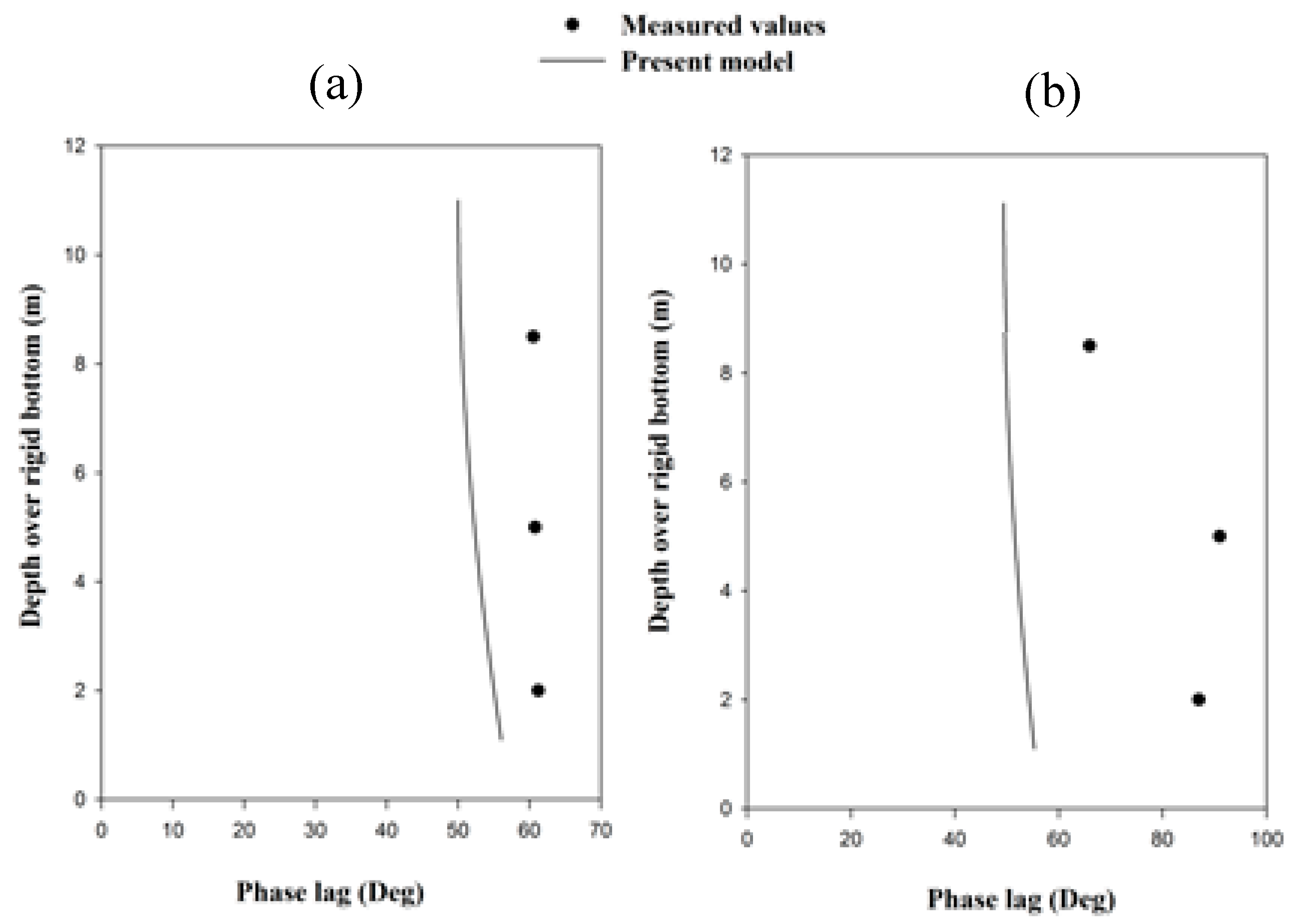
A comparison between the theoretical results of the mud particle velocities and the measured values presented by Soltanpour et al. [10] at y = 8.5 cm from the rigid bottom shows good agreements between the model results and laboratory data (Figure 15). Such an agreement is valid for the ranges of the high viscosity of the O (0.01 N/m²). This is because such high mud viscosities result in large boundary layer thicknesses of the mud layer that matches well with the assumptions of the proposed analytical model. (The same conclusion was provided by Shamsnia et al., [34]). It is revealed from the figure that the model provides agreements with the data in the upper layer of mud. This is also confirmed in Figure 16, where the model is validated with the data in three different mud depths. The results are closer to the laboratory data adjacent to the bottom and interface. This is due to the boundary layer assumption made in this study. Shamsnia et al. [34] have shown that the models with boundary layer assumptions provided better agreements with the laboratory data with higher values of mud velocities in comparison with all the other models (confirmed in the present study). However, small fluctuations-induced by the mud layer inhomogeneity-and rheological effects could not be considered by the theory. A comparison between samples of modelled instantaneous velocity profiles and the model and measurements of Soltanpour et al. [10] reveals that both models provide good agreements with the data of the mud layer, while discrepancies exist between the results of the model of Soltanpour et al. [10] and the measurements inside the water layer (Figure 17). However, the proposed model has provided closer results to the measurements, especially for water velocities. This is because, despite the model of Soltanpour et al. [10], the proposed model has considered the water boundary layer. Good agreements can be seen between the modelled phase lags and the measurements of Soltanpour et al. [10] for the two cases of following and opposing currents (Figure 18).

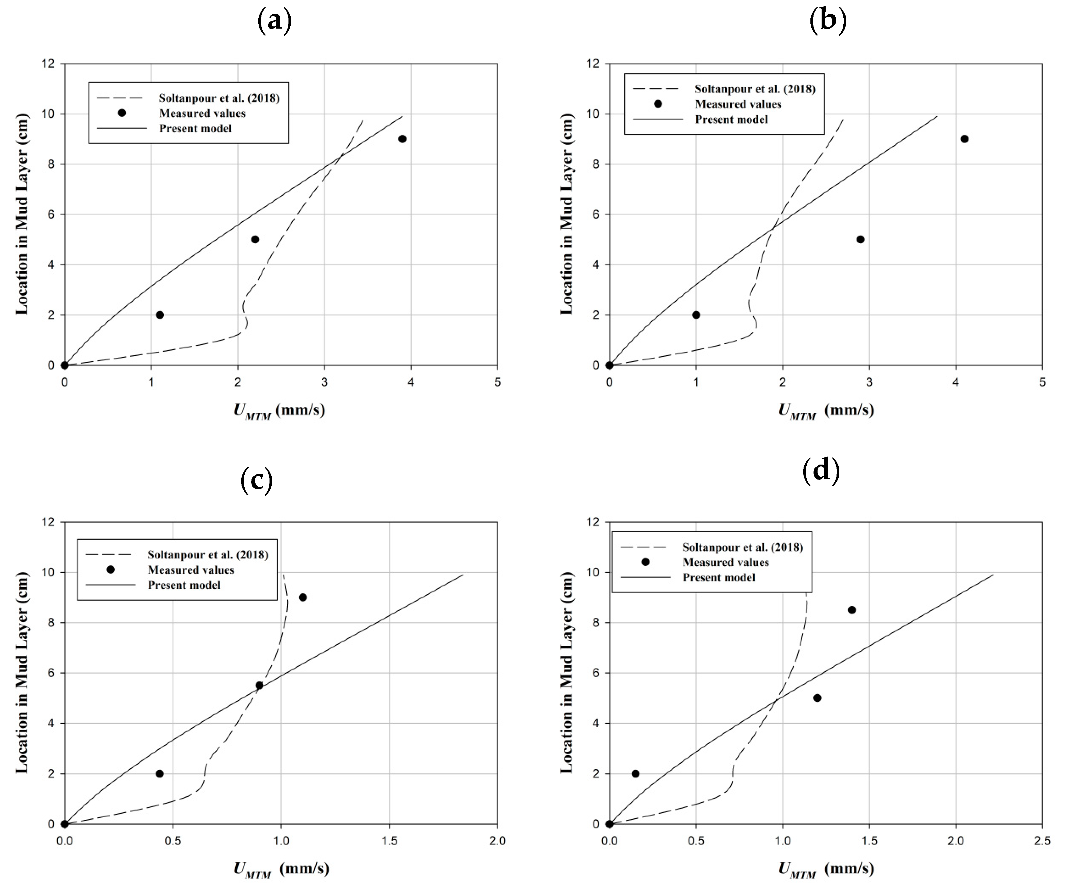
Comparisons between the modelled mud mass transport velocity profiles and the measured values of Soltanpour et al. [10] at three different vertical locations inside the mud layer; y = 2 cm, y = 5 cm, and y = 8.5 cm for the following and opposing current cases are provided with good agreements (Figure 19). The results of the Soltanpour et al. [10] model have also been compared with the results of the proposed model. Soltanpour et al. [10] found that the current does not penetrate the mud layer in the ranges of their current velocity (O(10 cm/s)) and mud viscosity (O(0.01 N/m²)). Therefore, due to the same assumption with their findings, the results of mass transport obtained from the proposed theory provide agreements with their experimental results. As also observed in the figure, the proposed model has provided closer results to the measurements compared to the model of Soltanpour et al. [10]. This shows that the proposed model assumptions of the boundary layer in the lower mud matches better with the real experimental conditions compared to the conventional complete and thin layer model of Dalrymple and Liu [11] that have been applied by many researchers (e.g., [10,12,26], etc.). It is also proved, more specifically, that the proposed model provides better agreements with the experimental data in comparison with the model of Soltanpour et al. [10] (Figure 20). The proposed model has lower values of relative differences compared to that of Soltanpour et al. [10] (

Table 5. Comparison of laboratory data, model of Soltanpour et al. [10] and proposed model outputs of mud mass transport velocity for co- and counter current cases. LD means laboratory data; PM means proposed model; SH means model of Soltanpour et al. [10]; RD means relative difference.

Following Current					Opposing Current
Mud Mass Transport Velocity (mm/s)			RDPM	RDSH	Mud Mass Transport Velocity (mm/s)			RDPM	RDSH
LD	PM	SH			LD	PM	SH
1.1	0.69	2.06	−0.37	0.87	0.439	0.31	0.65	−0.29	0.48
2.2	1.96	2.47	−0.11	0.12	0.9	0.92	0.91	0.02	0.01
3.9	3.31	3.11	−0.15	−0.2	1.1	1.38	1.01	0.25	−0.08
1	0.66	1.6	−0.34	0.6	0.15	0.36	0.71	1.4	3.73
2.9	1.91	1.9	−0.34	−0.34	1.2	1.1	1.01	−0.08	−0.16
4.1	3.3	2.5	−0.19	−0.39	1.4	1.66	1.12	0.18	−0.2

). In the summaries of the measured and modeled results of the mud mass transport velocities (Table 5), relative difference = (model outputs-experimental results)/experimental results.

3.2.2. Second Test Case

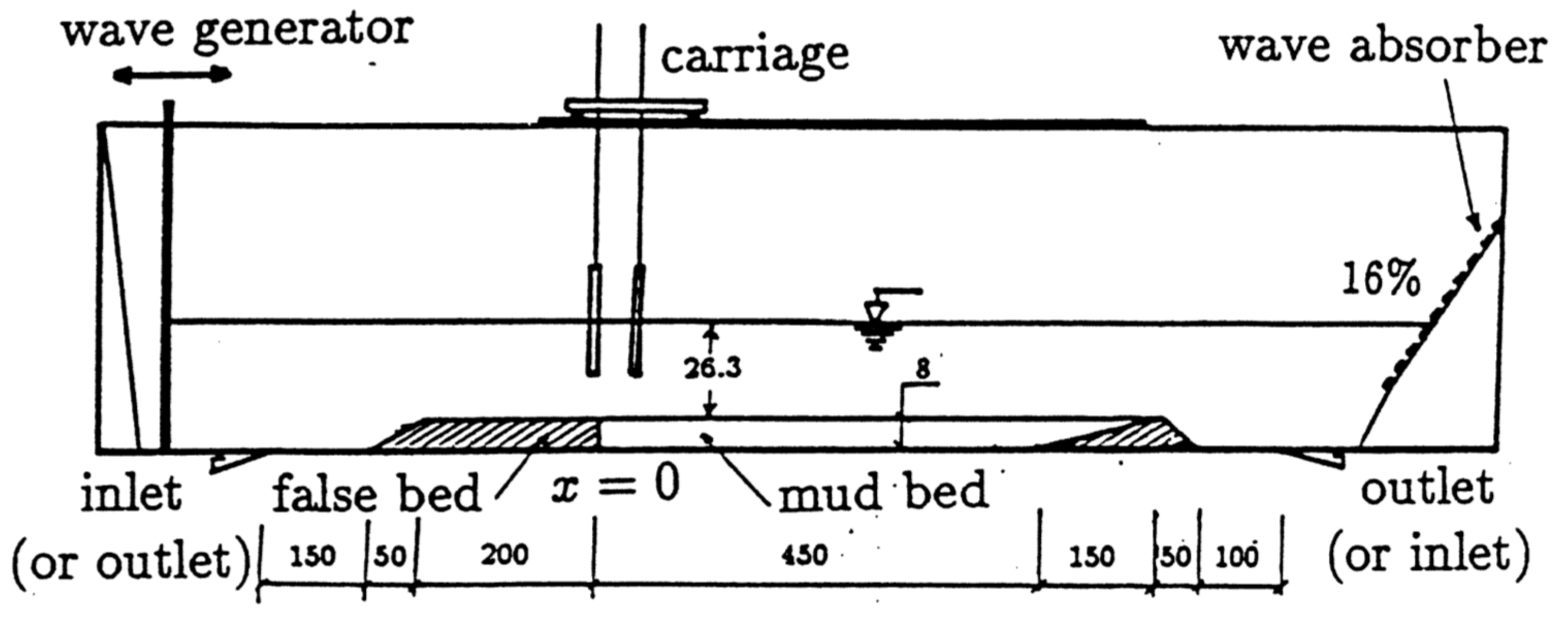
In this section, the results of laboratory experiments carried by An and Shibayama [26] have been used for the verification of the proposed analytical model. A mixture of kaolinite and tap water was used as the fluid mud layer with a thickness of 0.08 m. The flume was then slowly filled with tap water, up to a total depth of 0.343 m (Figure 21). The wave heights were measured using electric capacitance wave gauges (two sensors with a distance of 50 cm). Both opposing and following currents were applied in the experimental conditions with the wave periods and wave amplitudes being in the ranges similar to that of Soltanpour et al. [10] (

Table 6. Laboratory experiments conditions [26]. The parameter a₂ is the wave amplitude recorded by the second sensor (with 0.5 m distance to the first sensor). LD means laboratory data; PM means proposed model; RD means relative difference.

No.	T (s)	a (m)	Water Content Ratio (%)	U (m/s)	a2/a
					PM	LD	RD (%)
WC5	1.0	0.0224	158	−0.1911	0.96	0.95	0.4
WC6	1.1	0.0224	158	−0.09	0.97	0.96	1.05
WC8	1.2	0.0224	158	0.081	0.98	0.96	0.7
WC9	1.2	0.0224	158	0.1864	0.98	0.97	0.65

).

The results of the proposed model in the prediction of the dissipated wave amplitudes are acceptable (with small relative differences, e.g., lower than 2%) (Table 6). Slight discrepancies are due to the mud inhomogeneity during the experiments or the current profile variations due to the wave tilting. As seen in the results, the proposed model shows better agreement with the laboratory data in dissipation rates compared to the results of mud mass transport velocities (e.g., Table 5). This is because the mud mass transport velocities are second-order quantities with smaller orders of magnitudes compared to the wave amplitudes ([15,25]). Besides, some uncertainties, such as the mud thixotropic behaviors, or inhomogeneity, exist in the measurements, which are not considered in the analytical/numerical models.

4. Conclusions

This study provides an analytical investigation of wave–current–mud interaction. The proposed model can be used in the prediction of mud transport where the waves and currents coexist (e.g., confluences of rivers, estuaries, and seas). By the estimation of the mud transport over several periods, pollutant species transports can be calculated, and dredging volumes are estimated that both help the environmental/water scientists and engineers to preserve and manage the coasts and ports. The perturbation approach was adopted to solve the water–mud system of equations to the second order. The effects of current on particle velocity, dissipation rates, and phase shift in the first order and the mass transport and mean velocity in the second-order were investigated. The results of the model have been compared with the measured values of Soltanpour et al. [10], and An and Shibayama [26]. In addition to the fact that the proposed model provides explicit and straightforward expressions for the mud particle and mass transport velocities for the first time, the results show that the proposed model has superiority to the model of Soltanpour et al. [10] in the calculation of mud mass transport velocity. Good agreements are achieved in the calculations of the mud induced wave height attenuation in the presence of currents when compared with the measurements of An and Shibayama [26]. The following results were achieved from the present study:

• The following current decreases the particle velocity and dissipation rates, while the phase shift may increase, decrease, or be constant by moving from the opposing current to the following current.
• In the second-order, the mud mass transport is increased by a shift from opposing to following currents.
• Particle velocity, dissipation rates, and phase shift show a local peak versus the dimensionless mud thickness.
• The proposed assumption of a thin mud layer, which depth is in the same order as its boundary layer thickness matches better with the laboratory data in the mud viscosity of the orders of (0.01 N/m²) compared to the models in the literature.

A more general study must be carried to investigate the effects of the lower values of current velocities on mud mass transport (e.g., when the current velocity is of the same order as the wave-induced velocities). Attempts also must be made to generalize the present study assumption to find the ranges of viscosity that make the mud softer and the current to penetrate the mud layer.

References

- Zhao, Z.D.; Lian, J.J.; Shi, J.Z. Interactions among waves, current, and mud: Numerical and laboratory studies. J. Adv. Water Resour. 2006, 29, 1731–1744. [Google Scholar] [CrossRef]
- Sheremet, A.; Stone, G.W. Observations of nearshore wave dissipation over muddy sea beds. J. Geophys. Res. Oceans 2003, 108. [Google Scholar] [CrossRef]
- Rogers, W.E.; Holland, K.T. A study of dissipation of wind-waves by mud at Cassino Beach, Brazil: Prediction and inversion. Cont. Shelf Res. 2009, 29, 676–690. [Google Scholar] [CrossRef]
- Wells, J.T. Dynamics of coastal fluid muds in low-, moderate-, and high-tide-range environments. Can. J. Fish. Aquat. Sci. 1983, 40, s130–s142. [Google Scholar] [CrossRef]
- Haghshenas, S.A.; Soltanpour, M. An analysis of wave dissipation at the Hendijan mud coast, the Persian Gulf. Ocean Dyn. 2011, 61, 217–232. [Google Scholar] [CrossRef]
- Schulz, K.; Burchard, H.; Mohrholz, V.; Holtermann, P.; Schuttelaars, H.M.; Becker, M.; Gerkema, T. Intratidal and spatial variability over a slope in the Ems estuary: Robust along-channel SPM transport versus episodic events. Estuar. Coast. Shelf Sci. 2020, 243, 106902. [Google Scholar] [CrossRef]
- Levasseur, A. Observations and Modelling of the Variability of the Solent-Southampton Water Estuarine System. Ph.D. Thesis, University of Southampton, Southampton, UK, 2008. [Google Scholar]
- Hsu, W.Y.; Hwung, H.H.; Hsu, T.J.; Torres-Freyermuth, A.; Yang, R.Y. An experimental and numerical investigation on wave-mud interactions. J. Geophys. Res. Oceans 2013, 118, 1126–1141. [Google Scholar] [CrossRef]
- Ng, C.O. Mass transport in a layer of power-law fluid forced by periodic surface pressure. Wave Motion 2004, 39, 241–259. [Google Scholar] [CrossRef]
- Soltanpour, M.; Shamsnia, S.H.; Shibayama, T.; Nakamura, R. A study on mud particle velocities and mass transport in wave-current-mud interaction. Appl. Ocean Res. 2018, 78, 267–280. [Google Scholar] [CrossRef]
- Dalrymple, R.A.; Liu, P.L.-F. Waves over soft mud: A two-layer fluid model. J. Phys. Oceanogr. 1978, 8, 1121–1131. [Google Scholar] [CrossRef] [Green Version]
- Macpherson, H. The attenuation of water waves over a non-rigid bed. J. Fluid Mech. 1980, 97, 721–742. [Google Scholar] [CrossRef]
- Xia, Y.Z. The attenuation of shallow-water waves over seabed mud of a stratified viscoelastic model. Coast. Eng. J. 2014, 56, 1450021. [Google Scholar] [CrossRef]
- Dore, B.D. Mass transport in layered fluid systems. J. Fluid Mech. 1970, 40, 113–126. [Google Scholar] [CrossRef]
- Ng, C.O. Water waves over a muddy bed: A two-layer stokes boundary layer model. J. Coast. Eng. 2000, 40, 221–242. [Google Scholar] [CrossRef]
- Ng, C.O. Mass transport and set-ups due to partial standing surface waves in a two-layer viscous system. J. Fluid Mech. 2004, 520, 297–325. [Google Scholar] [CrossRef] [Green Version]
- Alam, M.R. Interaction of Waves in a Two-Layer Density Stratified Fluid. Ph.D. Thesis, Massachusetts Institute of Technology, Cambridge, MA, USA, 2008. [Google Scholar]
- Shen, X.; Toorman, E.A.; Fettweis, M.; Lee, B.J.; He, Q. Simulating multimodal floc size distributions of suspended cohesive sediments with lognormal subordinates: Comparison with mixing jar and settling column experiments. J. Coast. Eng. 2019, 148, 36–48. [Google Scholar] [CrossRef]
- Dijkstra, Y.M.; Schuttelaars, H.M.; Schramkowski, G.P.; Brouwer, R.L. Modeling the transition to high sediment concentrations as a response to channel deepening in the Ems River Estuary. J. Geophys. Res. Oceans 2019, 124, 1578–1594. [Google Scholar] [CrossRef] [Green Version]
- Gade, H.G. Effects of a nonrigid, impermeable bottom on plane surface waves in shallow water. J. Mar. Res. 1958, 16, 61–82. [Google Scholar]
- Piedra Cueva, I. On the response of a muddy bottom to surface water waves. J. Hydraul. Res. 1993, 31, 681–696. [Google Scholar] [CrossRef]
- Liu, P.L.F.; Chan, I.C. A note on the effects of a thin visco-elastic mud layer on small amplitude water-wave propagation. J. Coast. Eng. 2007, 54, 233–247. [Google Scholar] [CrossRef]
- Kranenburg, W.M.; Winterwerp, J.C.; de Boer, G.J.; Cornelisse, J.M.; Zijlema, M. SWAN-Mud: Engineering model for mud-induced wave damping. J. Hydraul. Eng. 2011, 137, 959–975. [Google Scholar] [CrossRef]
- Ng, C.O.; Zhang, X. Mass transport in water waves over a thin layer of soft viscoelastic mud. J. Fluid Mech. 2007, 573, 105–130. [Google Scholar] [CrossRef] [Green Version]
- Sakakiyama, T.; Bijker, E.W. Mass transport velocity in mud layer due to progressive waves. J. Waterw. Port Coast. Ocean Eng. 1989, 115, 614–633. [Google Scholar] [CrossRef]
- An, N.N.; Shibayama, T. Wave-current interaction with mud bed. In Proceedings of the Coastal Engineering, ASCE, Kobe, Japan, 23–28 October 1994; Volume 1, pp. 2913–2927. [Google Scholar]
- Zhang, D.-H.; Ng, C.-O. A numerical study on wave–mud interaction. China Ocean Eng. 2006, 20, 383–394. [Google Scholar]
- Niu, X.; Yu, X. A numerical model for wave propagation over muddy slope. Coast. Eng. Proc. 2011, 1, waves-27. [Google Scholar] [CrossRef]
- Jiang, L.; Zhao, Z. Viscous damping of solitary waves over fluid-mud seabeds. J. Waterw. Port Coast. Ocean Eng. 1989, 115, 345–362. [Google Scholar] [CrossRef]
- Huang, L.; Chen, Q. Spectral collocation model for solitary wave attenuation and mass transport over viscous mud. J. Eng. Mech. 2009, 135, 881–891. [Google Scholar] [CrossRef]
- Park, Y.S.; Liu, P.L.; Clark, S.J. Viscous flows in a muddy seabed induced by a solitary wave. J. Fluid Mech. 2008, 598, 383. [Google Scholar] [CrossRef]
- Chan, I.C.; Liu, P.L. Responses of Bingham-plastic muddy seabed to a surface solitary wave. J. Fluid Mech. 2009, 618, 155. [Google Scholar] [CrossRef]
- Samsami, F.; Soltanpour, M.; Shibayama, T. Spectral analysis of irregular waves in wave-mud and wave-current-mud interactions. J. Ocean Dyn. 2015, 65, 1305–1320. [Google Scholar] [CrossRef]
- Shamsnia, S.H.; Soltanpour, M.; Bavandpour, M.; Gualtieri, C. A study of wave dissipation rate and particles velocity in muddy beds. Geosciences 2019, 9, 212. [Google Scholar] [CrossRef] [Green Version]
- Nakano, S. Wave Damping and Mud Transport. Ph.D. Thesis, Kyoto University, Kyoto, Japan, 1994; p. 212. (In Japanese). [Google Scholar]
- Longuet-Higgins, M.S. Mass transport in water waves. Phil. Trans. R. Soc. Lond. A 1953, 245, 535–581. [Google Scholar]
- Maa, J.P.Y.; Mehta, A.J. Soft mud response to water waves. J. Waterw. Port Coast. Ocean Eng. 1990, 116, 634–650. [Google Scholar] [CrossRef]
Figure 1.
A schematic view of the wave–current–mud interaction problem (modified from [5]).
Figure 2.
Particle velocity profiles for different following, opposing, and no current conditions, (a) 10; (b) 100.
Figure 3.
Particle velocity amplitudes versus current velocity at different depth in the mud layer.
Figure 4.
Particle velocity amplitudes versus dimensionless mud thickness, dN, (a) y = 0.9d; (b) y = 0.5d; (c) y = 0.2d.
Figure 5.
Dissipation rates versus current velocity, U.
Figure 6.
Dissipation rates versus dimensionless mud thickness, dN.
Figure 7.
Dissipation rates versus wave period, T.
Figure 8.
Phase shift profile in mud depth for different current velocities.
Figure 9.
Phase shift versus current velocity for different values of ζ.
Figure 10.
Phase shift versus dimensionless mud thickness, dN.
Figure 11.
Phase shift versus ζ.
Figure 12.
Mud mass transport velocity profile for different values of current velocity.
Figure 13.
Mud mass transport rate, Q versus dimensionless mud thickness, dN for different types of following current, no current, and opposing current conditions.
Figure 14.
Experimental set-ups and boundary conditions (T1–T8) (modified from Soltanpour et al. [10]).
Figure 15.
Comparison of particle velocity time series of the theory with the measured values of Soltanpour et al. [10], y = 8.5 cm; (a) T = 1.2 s, a = 2 cm, U = 7 cm/s; (b) T = 1.2 s, a = 2 cm; (c) T = 1.2 s, a = 2 cm, U = −10 cm/s.
Figure 16.
Comparison of particle velocity time series of the theory with the measured values of Soltanpour et al. [10], T = 1.1 s, a = 2.33 cm, U = 9.85 cm/s; (a) y = 2.0 cm; (b) y = 5.0 cm; (c) y = 8.5 cm.
Figure 17.
Comparison of instantaneous velocities of the present model, Soltanpour et al. [10], and the measured values of Soltanpour et al. [10] under the crest (a,c); and under the through (b,d), y = 8.5 cm; (a,b) T = 1.1 s; a = 2.33 cm, U = 9.85 cm/s; (c,d) T = 1.1 s, a = 2.485 cm, U = −7.47 cm/s.
Figure 18.
Comparison of phase lags of the theory (curve lines) with the measured values (dots) of Soltanpour et al. [10], y = 8.5 cm; (a) T = 1.1 s; a = 2.33 cm, U = 9.85 cm/s; (b) T = 1.1 s; a = 2.485 cm, U = −7.47 cm/s.
Figure 19.
Comparison of the mud mass transport of the theory with the measured values of Soltanpour et al. [10] (y = 8.5 cm); (a) T = 1.2 s, a = 3.32 cm, U = 4.71 cm/s; (b) T = 1.2 s, a = 3.39 cm, U = 10.17 cm/s; (c) T = 1.2 s, a = 2.02 cm, U = −6.65 cm/s; (d) T = 1.2 s, a = 2.1 cm, U = −10.75 cm/s.
Figure 20.
Measured via modelled mud mass transport velocities from proposed model and model of Soltanpour et al. [10].
Figure 21.
Experimental set-up (after An and Shibayama [26]).