Evaluation of Different Objective Functions Used in the SUFI-2 Calibration Process of SWAT-CUP on Water Balance Analysis: A Case Study of the Pursat River Basin, Cambodia

 , and
, and
Abstract
:1. Introduction
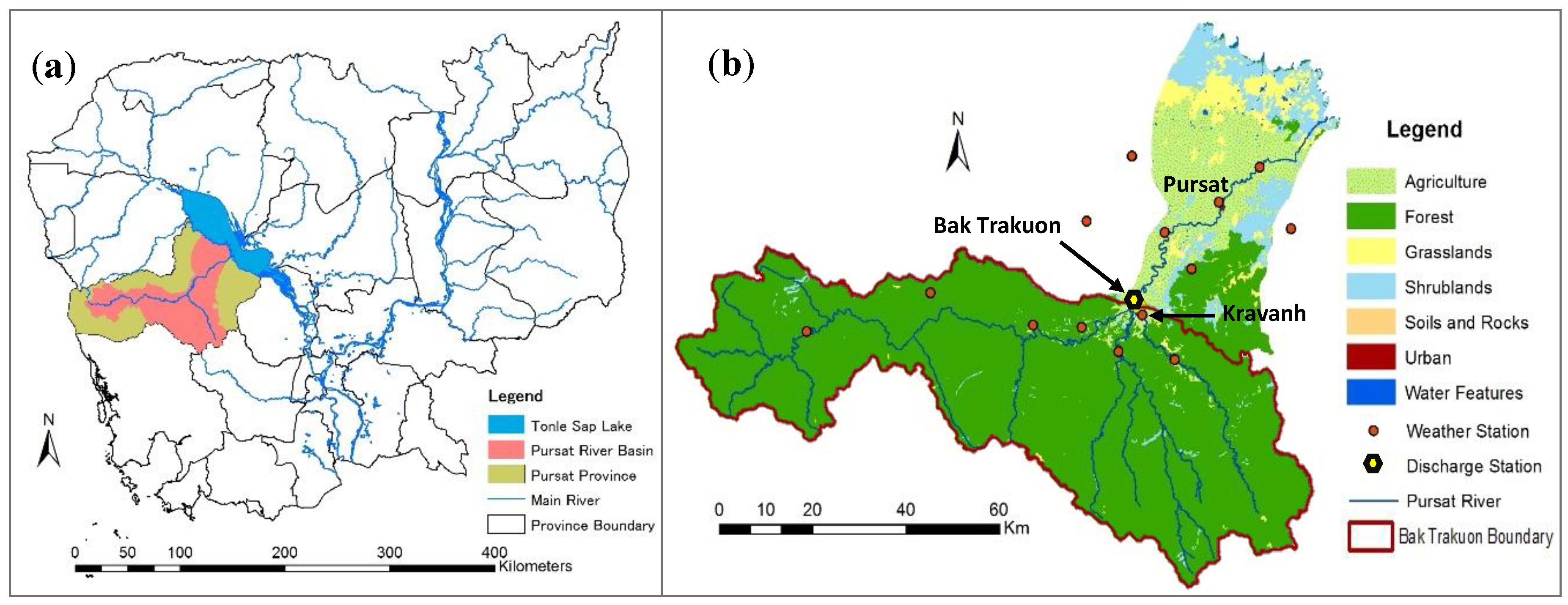
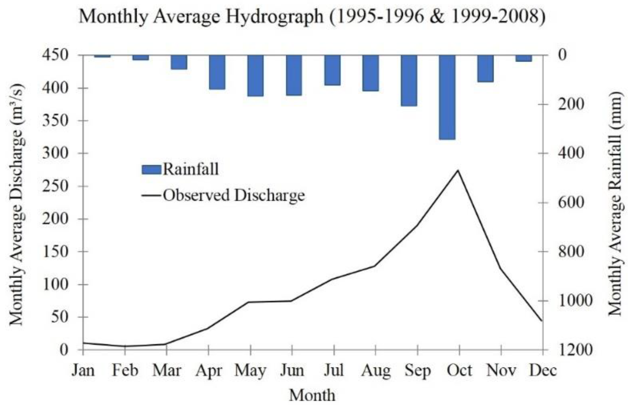
2. Study Area
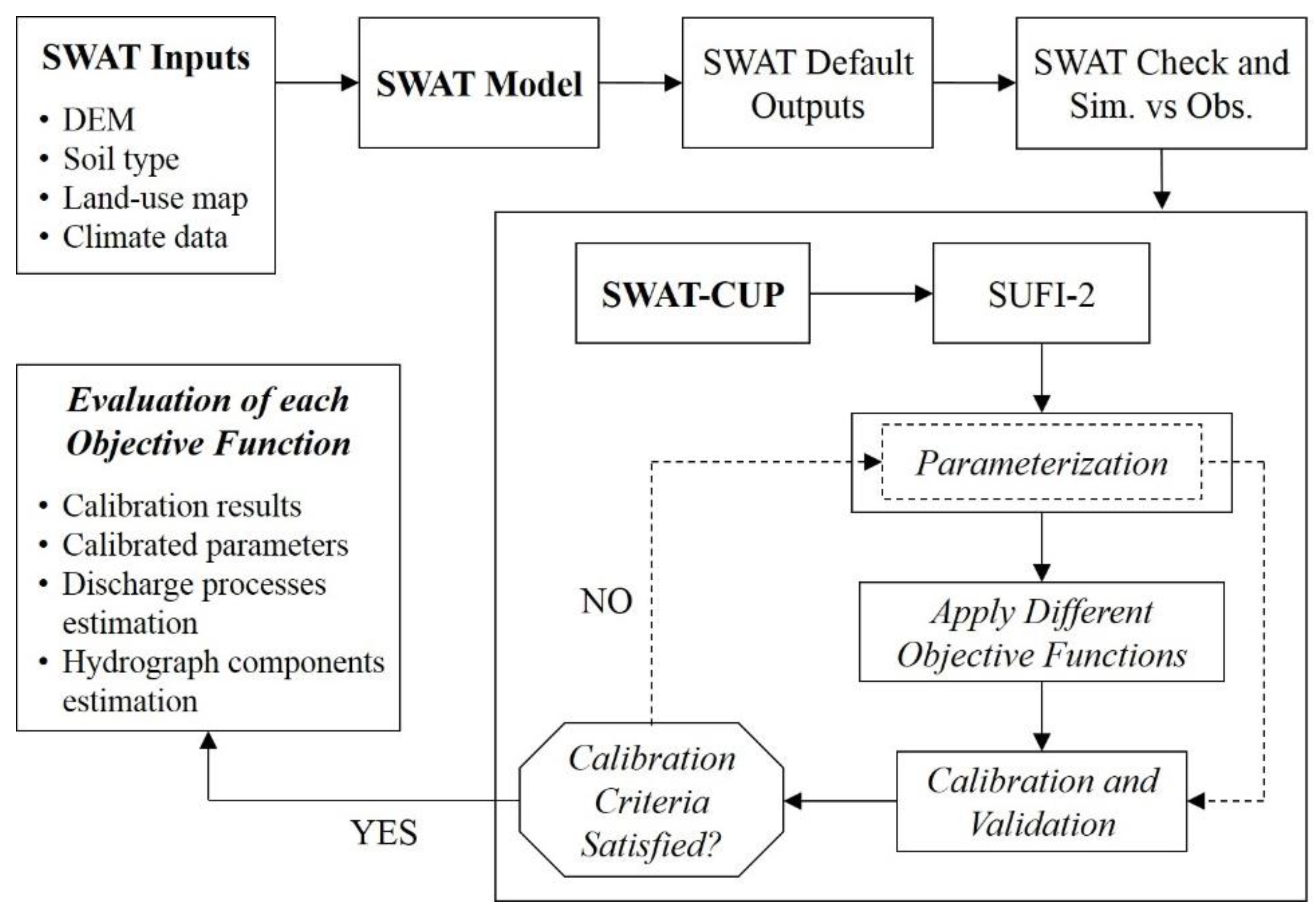
3. Materials and Methods
3.1. SWAT Input Datasets
3.2. SWAT Model Setup
3.3. SWAT-CUP with the SUFI-2 Algorithm
3.3.1. Parameterization
3.3.2. Objective Functions
3.3.3. Model Calibration, Validation, and Evaluation
3.4. Evaluation of Each Objective Function
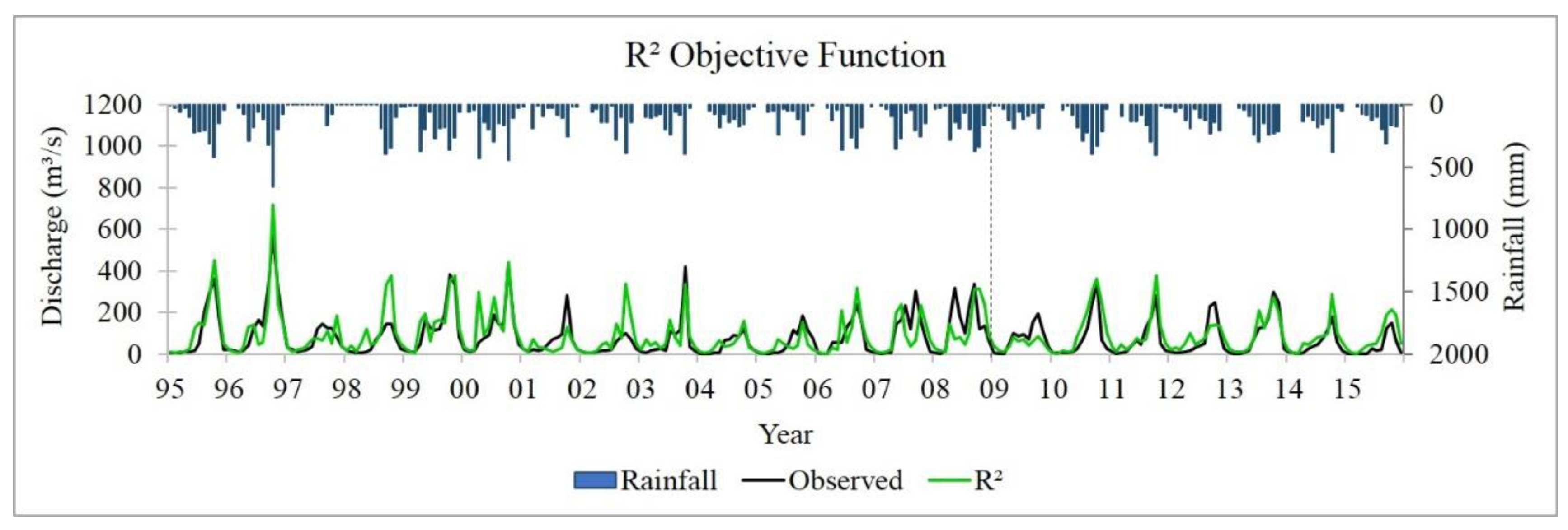
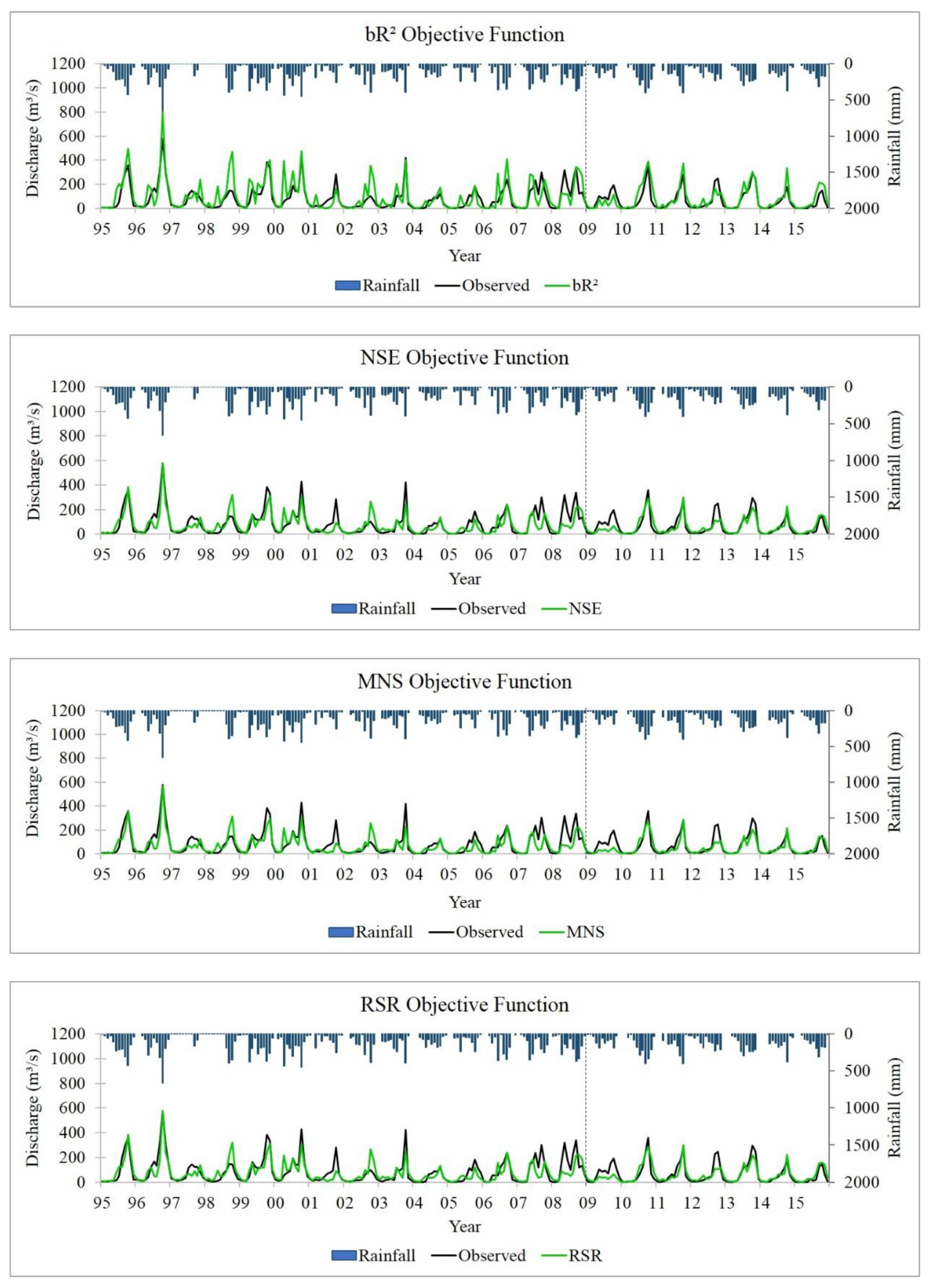
4. Results
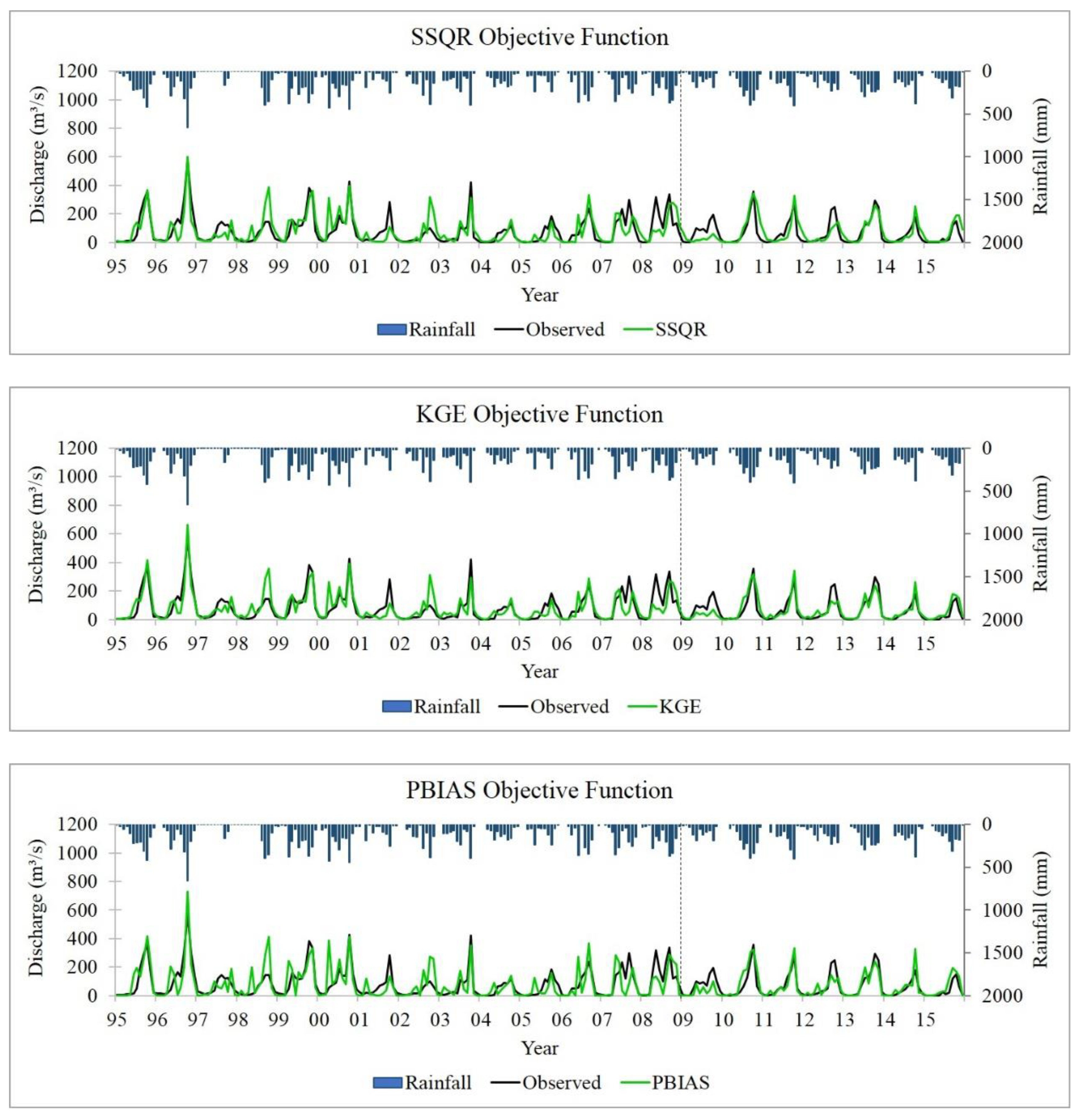
4.1. Simulation Results
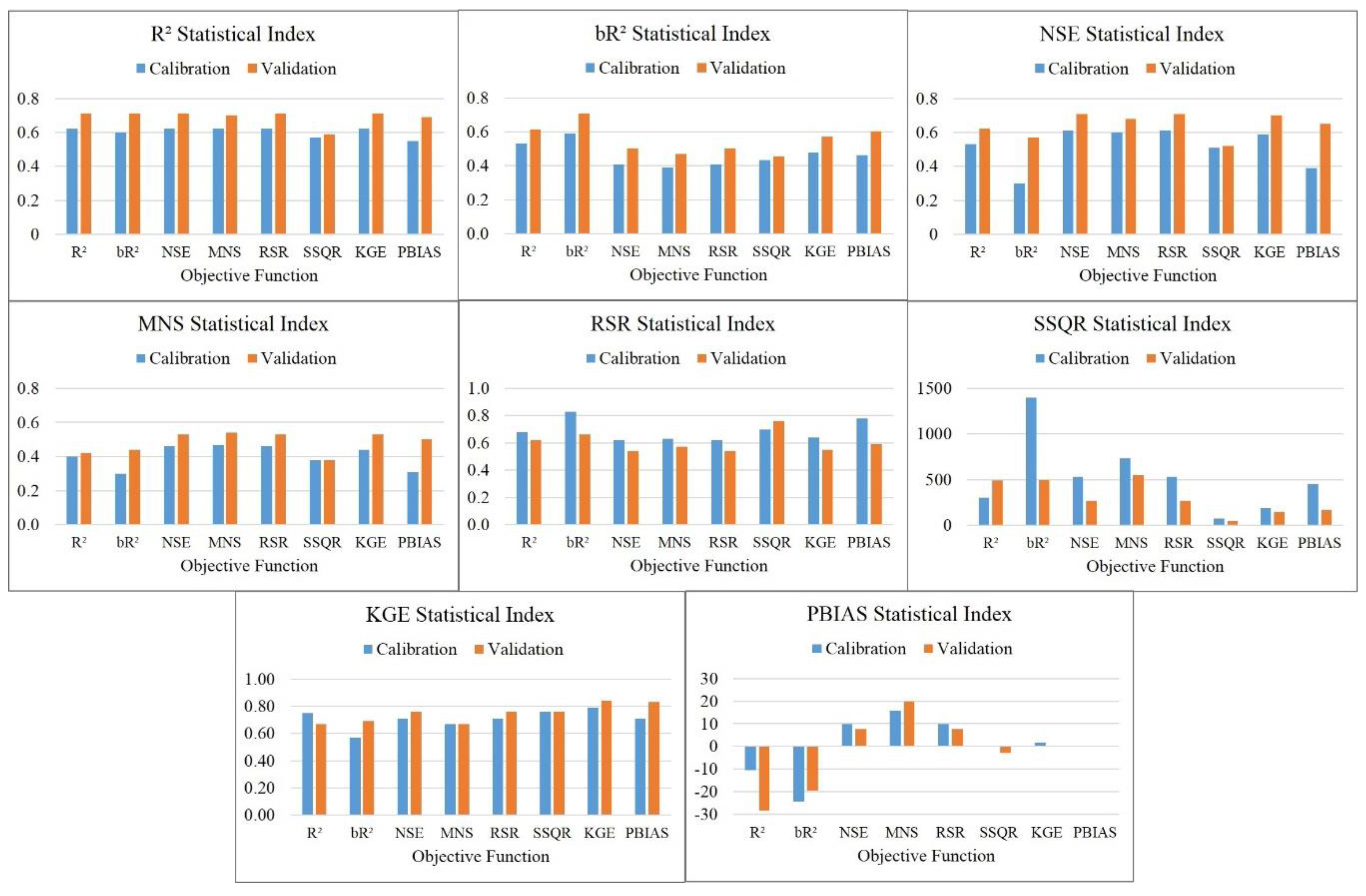
4.2. Model Performance
5. Discussion
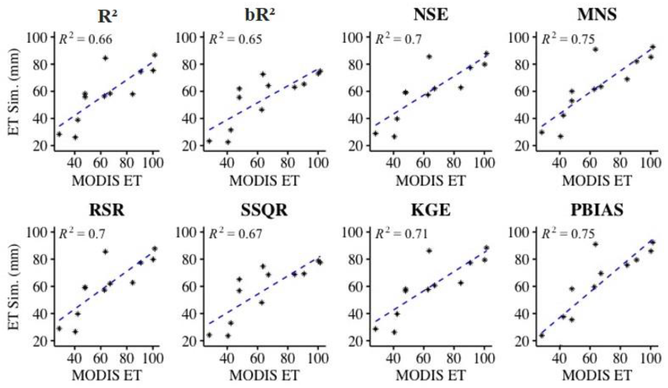
5.1. Discharge Process Estimations
5.2. Best Parameter Sets and Sensitivity Rank
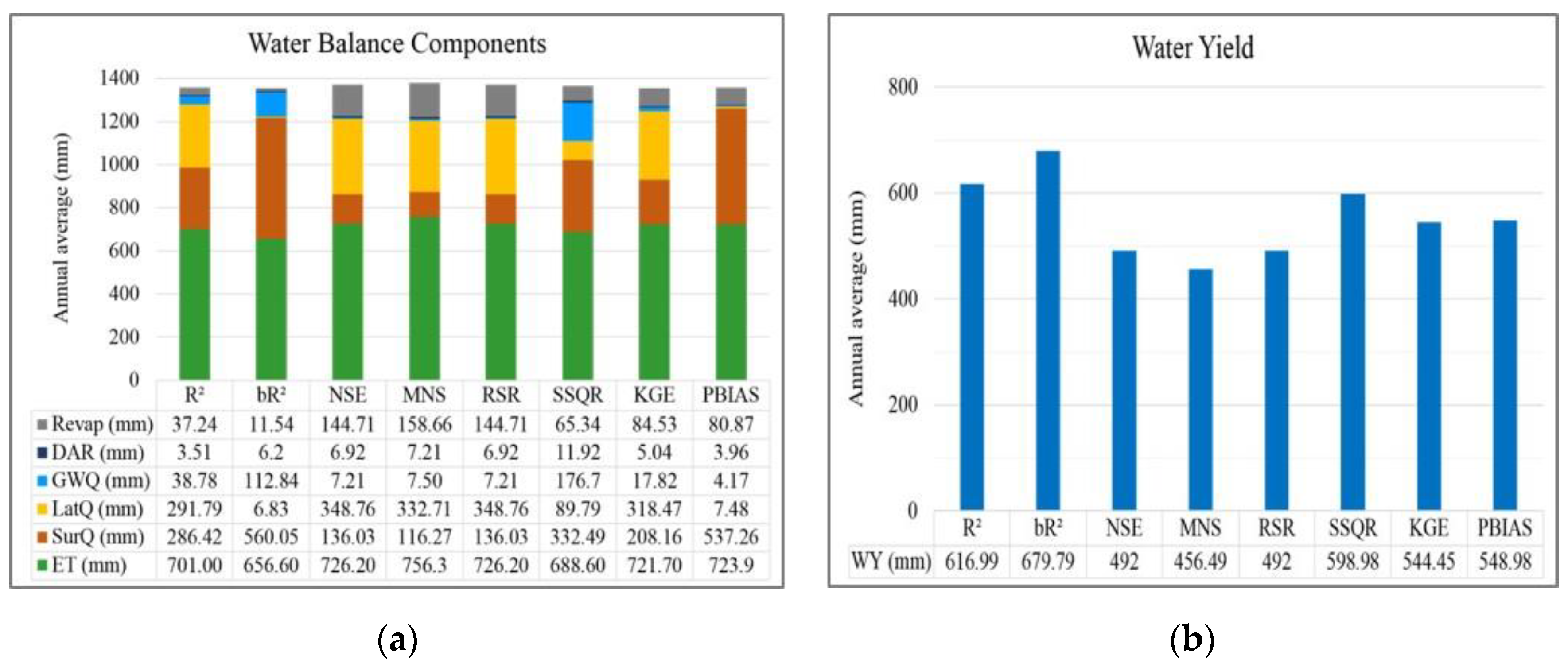
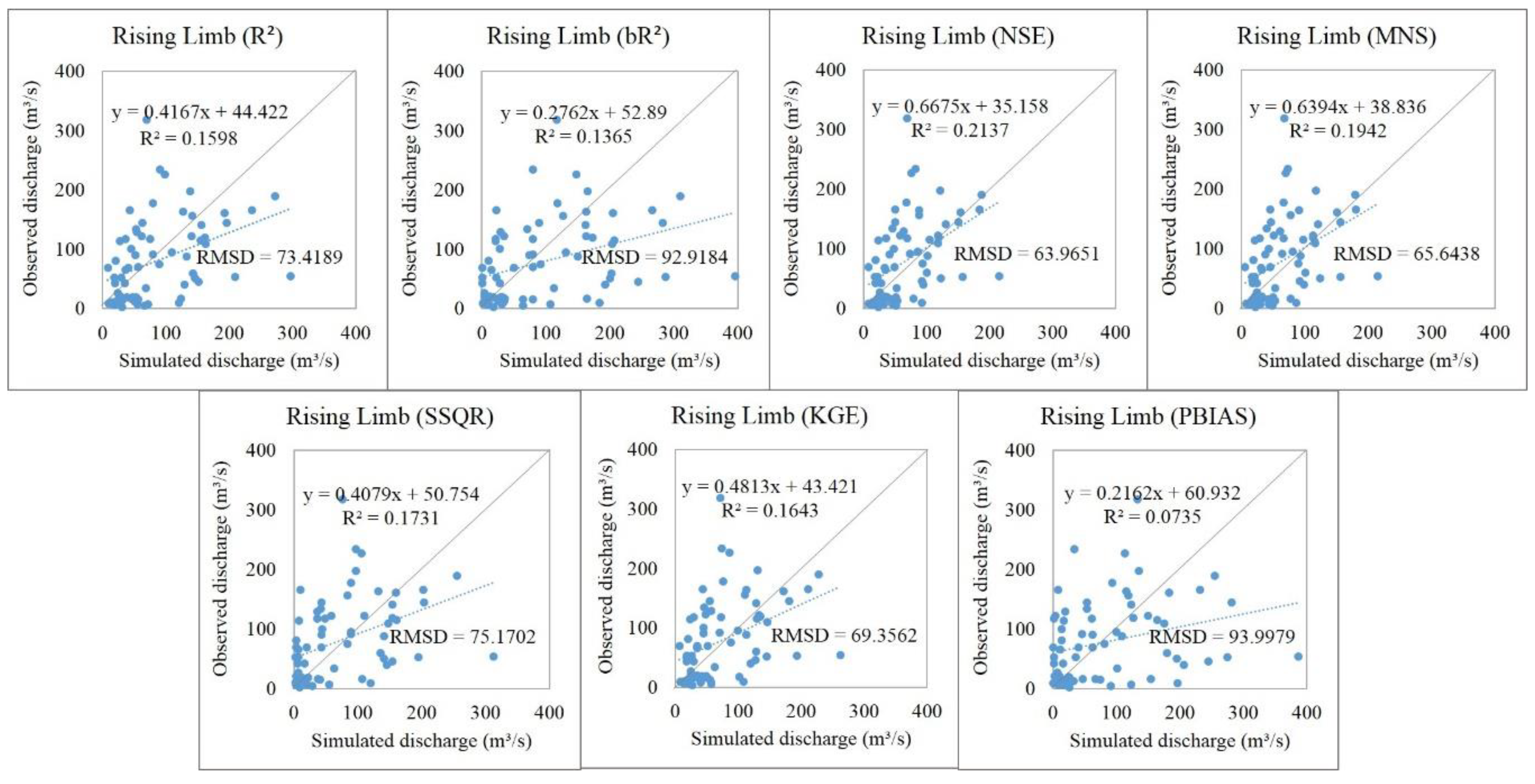
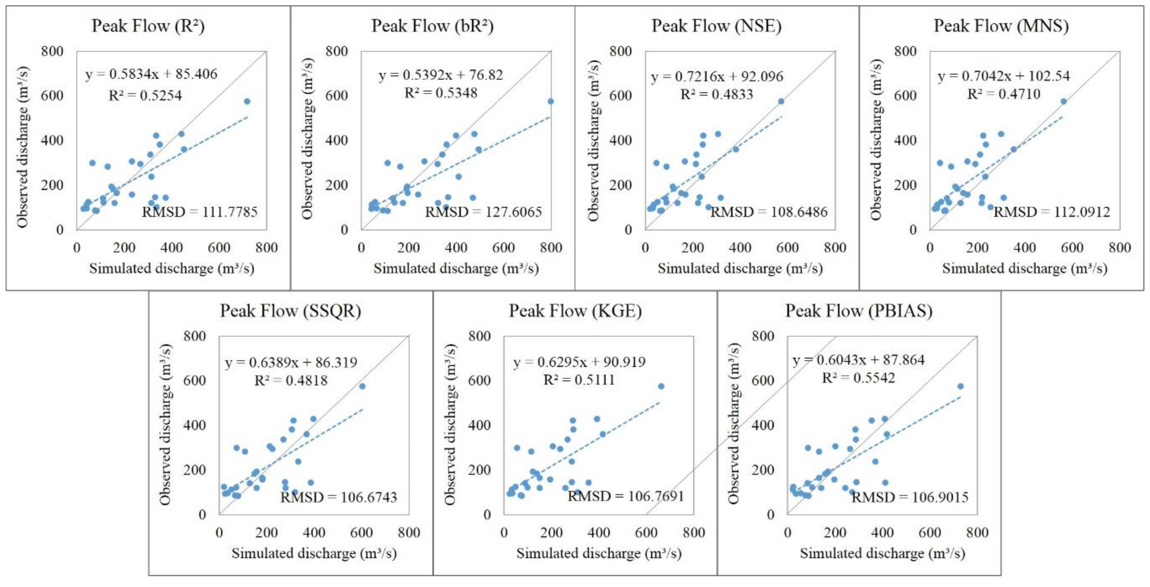
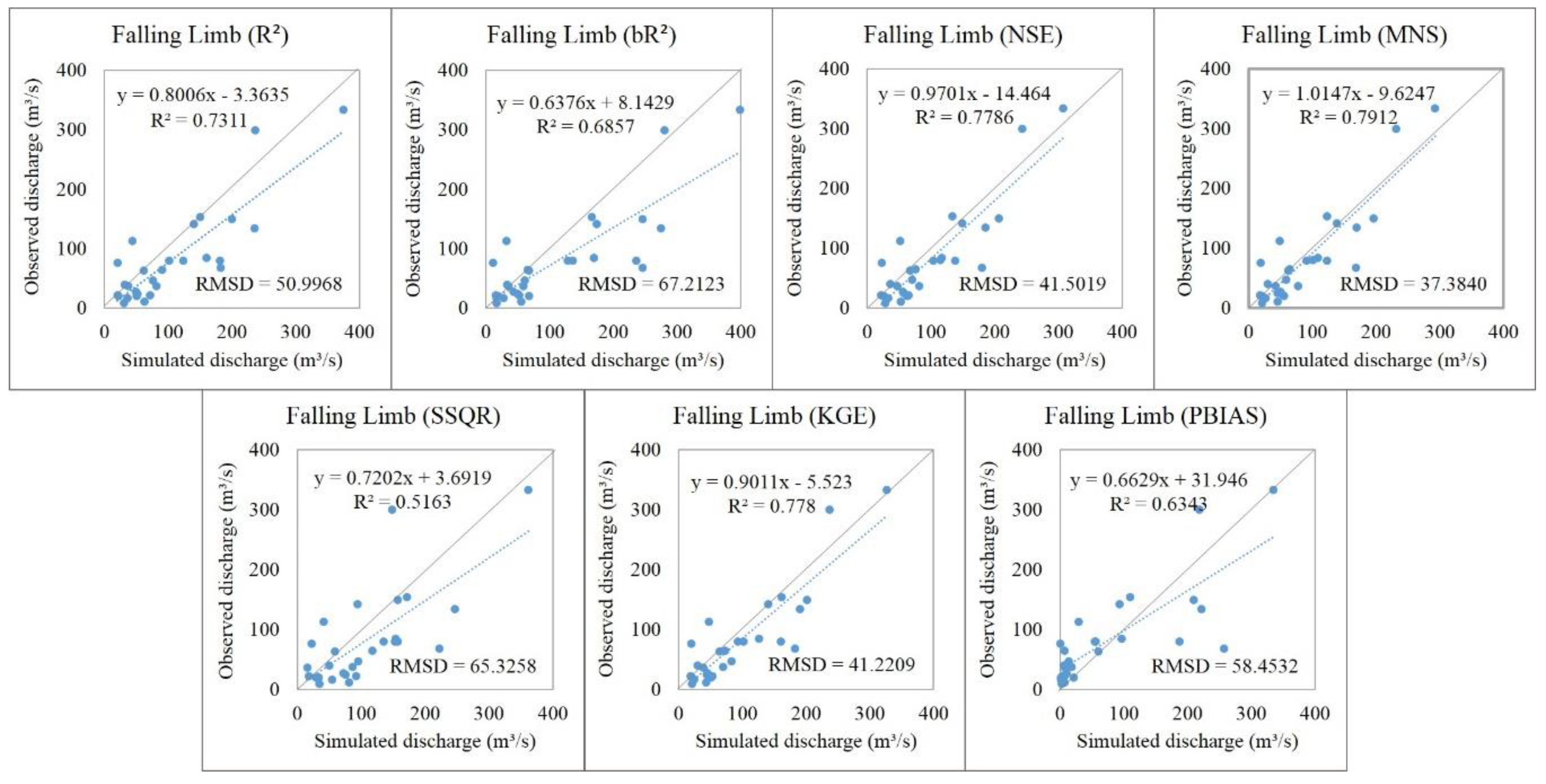
5.3. Hydrograph Components Estimation
5.4. Objective Functions Corresponding to the Characteristics of the River Basin
6. Conclusions
Author Contributions
Funding
Acknowledgments
Conflicts of Interest
References
- Gosain, A.K.; Rao, S.; Basuray, D. Climate change impact assessment on hydrology of Indian river basins. Curr. Sci. 2006, 90, 9. [Google Scholar]
- Rostamian, R.; Jaleh, A.; Afyuni, M.; Mousavi, S.F.; Heidarpour, M.; Jalalian, A.; Abbaspour, K.C. Application of a SWAT model for estimating runoff and sediment in two mountainous basins in central Iran. Hydrol. Sci. J. 2008, 53, 977–988. [Google Scholar] [CrossRef]
- Huang, T.; Lo, K. Effects of Land Use Change on Sediment and Water Yields in Yang Ming Shan National Park, Taiwan. Environments 2015, 2, 32–42. [Google Scholar] [CrossRef] [Green Version]
- Näschen, K.; Diekkrüger, B.; Evers, M.; Höllermann, B.; Steinbach, S.; Thonfeld, F. The Impact of Land Use/Land Cover Change (LULCC) on Water Resources in a Tropical Catchment in Tanzania under Different Climate Change Scenarios. Sustainability 2019, 11, 7083. [Google Scholar] [CrossRef] [Green Version]
- Cambien, N.; Gobeyn, S.; Nolivos, I.; Forio, M.A.E.; Arias-Hidalgo, M.; Dominguez-Granda, L.; Witing, F.; Volk, M.; Goethals, P.L.M. Using the Soil and Water Assessment Tool to Simulate the Pesticide Dynamics in the Data Scarce Guayas River Basin, Ecuador. Water 2020, 12, 696. [Google Scholar] [CrossRef] [Green Version]
- Arnold, J.G.; Srinivasan, R.; Muttiah, R.S.; Williams, J.R. Large area hydrologic modeling and assessment, Part I: Model development. J. Am. Water Resour. Assoc. 1998, 34, 73–89. [Google Scholar] [CrossRef]
- Arnold, J.G.; Moriasi, D.N.; Gassman, P.W.; Abbaspour, K.C.; White, M.J.; Srinivasan, R.; Santhi, C.; Harmel, R.D.; Van Griensven, A.; Van Liew, M.W.; et al. SWAT: Model Use, Calibration, and Validation. Trans. ASABE 2012, 55, 1491–1508. [Google Scholar] [CrossRef]
- Neitsch, S.L.; Arnold, J.G.; Kiniry, J.R.; Williams, J.R. Soil and Water Assessment Tool—Theoretical Documentation (Version 2005); Agricultural Research Service: Temple, TX, USA, 2005.
- Neitsch, S.L.; Arnold, J.G.; Kiniry, J.R.; Williams, J.R. Soil and Water Assessment Tool Theoretical Documentation Version 2009; Texas Water Resources Institute Technical Report No. 406; Texas A&M University System: College Station, TX, USA, 2011. [Google Scholar]
- Gassman, P.W.; Reyes, M.R.; Green, C.H.; Arnold, J.G. The Soil and Water Assessment Tool: Historical Development, Applications, and Future Research Directions. Trans. ASABE 2007, 50, 1211–1250. [Google Scholar] [CrossRef] [Green Version]
- Abbaspour, K.C.; Rouholahnejad, E.; Vaghefi, S.; Srinivasan, R.; Yang, H.; Kløve, B. A continental-scale hydrology and water quality model for Europe: Calibration and uncertainty of a high-resolution large-scale SWAT model. J. Hydrol. 2015, 524, 733–752. [Google Scholar] [CrossRef] [Green Version]
- Abbaspour, K.C. SWAT-CUP: SWAT Calibration and Uncertainty Programs—A User Manual; Swiss Federal Institute of Aquatic Science and Technology: Zurich, Switzerland, 2015. [Google Scholar]
- Ha, L.T.; Bastiaanssen, W.G.M.; van Griensven, A.; van Dijk, A.I.J.M.; Senay, G.B. SWAT-CUP for Calibration of Spatially Distributed Hydrological Processes and Ecosystem Services in a Vietnamese River Basin Using Remote Sensing. Hydrol. Earth Syst. Sci. Discuss. 2017, 1–35. [Google Scholar] [CrossRef] [Green Version]
- Roth, V.; Nigussie, T.K.; Lemann, T. Model parameter transfer for streamflow and sediment loss prediction with SWAT in a tropical watershed. Environ. Earth Sci. 2016, 75, 1321. [Google Scholar] [CrossRef] [Green Version]
- Gholami, A.; Habibnejad Roshan, M.; Shahedi, K.; Vafakhah, M.; Solaymani, K. Hydrological stream flow modeling in the Talar catchment (central section of the Alborz Mountains, north of Iran): Parameterization and uncertainty analysis using SWAT-CUP. J. Water Land Dev. 2016, 30, 57–69. [Google Scholar] [CrossRef]
- Abbaspour, K.C.; Vejdani, M.; Haghighat, S. SWAT-CUP Calibration and Uncertainty Programs for SWAT; Modelling and Simulation Society of Australia and New Zealand: Christchurch, New Zealand, 2007; pp. 1596–1602. [Google Scholar]
- Khoi, D.N.; Thom, V.T. Parameter uncertainty analysis for simulating streamflow in a river catchment of Vietnam. Glob. Ecol. Conserv. 2015, 4, 538–548. [Google Scholar] [CrossRef] [Green Version]
- Shivhare, N.; Dikshit, P.K.S.; Dwivedi, S.B. A Comparison of SWAT Model Calibration Techniques for Hydrological Modeling in the Ganga River Watershed. Engineering 2018, 4, 643–652. [Google Scholar] [CrossRef]
- Sloboda, M.; Swayne, D. Autocalibration of Environmental Process Models Using a PAC Learning Hypothesis. In Environmental Software Systems. Frameworks of eEnvironment; IFIP Advances in Information and Communication Technology; Springer: Berlin/Heidelberg, Germany, 2011; Volume 359, pp. 528–534. ISBN 978-3-642-22284-9. [Google Scholar]
- Kouchi, D.H.; Esmaili, K.; Faridhosseini, A.; Sanaeinejad, S.H.; Khalili, D.; Abbaspour, K.C. Sensitivity of Calibrated Parameters and Water Resource Estimates on Different Objective Functions and Optimization Algorithms. Water 2017, 9, 384. [Google Scholar] [CrossRef] [Green Version]
- Ashwell, D.; Lic, V.; Loeung, K.; Maltby, M.; McNaughton, A.; Mulligan, B.; Oum, S.; Starr, A. Baseline Assessment and Recommendations for Improved Natural Resources Management and Biodiversity Conservation in the Tonle Sap Basin, Cambodia; Fauna & Flora International: Phnom Penh, Cambodia, 2011; 92p. [Google Scholar]
- Cambodia National Mekong Committee (CNMC). Basin Development Plan Program (Ed.): Profile of the Tonle Sap Sub-Area (SA-9C); CNMC: Phnom Penh, Cambodia, 2012. [Google Scholar]
- Japan International Cooperation Agency (JICA). Report on Examination of Impact of New Dam Plans on the West Tonle Sap Irrigation Rehabilitation Project in Pursat River Basin; Ministry of Water Resources and Meteorology (MOWRAM): Phnom Penh, Cambodia, 2011. [Google Scholar]
- Japan International Cooperation Agency (JICA). Brief Progress Report on the Water Balance Examination Study for Pursat and Baribor River Basins; Ministry of Water Resources and Meteorology (MOWRAM): Phnom Penh, Cambodia, 2013. [Google Scholar]
- Abbaspour, K.C.; van Genuchten, M.T.; Schulin, R.; Schläppi, E. A sequential uncertainty domain inverse procedure for estimating subsurface flow and transport parameters. Water Resour. Res. 1997, 33, 1879–1892. [Google Scholar] [CrossRef] [Green Version]
- Abbaspour, K.C.; Johnson, C.A.; Van Genuchten, M.Th. Estimating Uncertain Flow and Transport Parameters Using a Sequential Uncertainty Fitting Procedure. Vadose Zone J. 2004, 3, 1340–1352. [Google Scholar] [CrossRef]
- Rossi, C.G.; Srinivasan, R.; Jirayoot, K.; Duc, T.L.; Souvannabouth, P.; Binh, N.; Gassman, P.W. Hydrologic Evaluation of the Lower Mekong River Basin with the Soil and Water Assessment Tool Model. Int. Agric. Eng. J. 2009, 18, 1–13. [Google Scholar]
- Ly, S.; Oeurng, C. Climate change and water governance in Stung Chrey Bak Cathment of Tonle Sap Great Lake Basin in Cambodia. In Proceedings of the 15th Annual Conference of the Science Council of Asia (SCA), Siem Reap, Cambodia, 17–19 May 2015; pp. 134–138. [Google Scholar]
- Ang, R.; Oeurng, C. Simulating streamflow in an ungauged catchment of Tonlesap Lake Basin in Cambodia using Soil and Water Assessment Tool (SWAT) model. Water Sci. 2018, 32, 89–101. [Google Scholar] [CrossRef] [Green Version]
- Krause, P.; Boyle, D.P.; Bäse, F. Comparison of different efficiency criteria for hydrological model assessment. Adv. Geosci. 2005, 5, 89–97. [Google Scholar] [CrossRef] [Green Version]
- Nash, J.E.; Sutcliffe, J.V. River flow forecasting through conceptual models part I—A discussion of principles. J. Hydrol. 1970, 10, 282–290. [Google Scholar] [CrossRef]
- Moriasi, D.N.; Arnold, J.G.; Liew, M.W.V.; Bingner, R.L.; Harmel, R.D.; Veith, T.L. Model Evaluation Guidelines for Systematic Quantification of Accuracy in Watershed Simulations. Trans. ASABE 2007, 50, 885–900. [Google Scholar] [CrossRef]
- Van Griensven, A.; Bauwens, W. Multiobjective autocalibration for semidistributed water quality models: Autocalibrations for water quality models. Water Resour. Res. 2003, 39, 1348. [Google Scholar] [CrossRef]
- Gupta, H.V.; Kling, H.; Yilmaz, K.K.; Martinez, G.F. Decomposition of the mean squared error and NSE performance criteria: Implications for improving hydrological modelling. J. Hydrol. 2009, 377, 80–91. [Google Scholar] [CrossRef] [Green Version]
- Yapo, P.O.; Gupta, H.V.; Sorooshian, S. Automatic calibration of conceptual rainfall-runoff models: Sensitivity to calibration data. J. Hydrol. 1996, 181, 23–48. [Google Scholar] [CrossRef]
- James, L.D.; Burges, S.J. Selection, Calibration, and Testing of Hydrologic Models. In Hydrologic Modeling of Small Watersheds; American Society of Agricultural Engineers: St. Joseph, MI, USA, 1982; pp. 437–470. [Google Scholar]
- Muleta, M.K. Model Performance Sensitivity to Objective Function during Automated Calibrations. J. Hydrol. Eng. 2012, 17, 756–767. [Google Scholar] [CrossRef]
- Mehdi, B.; Ludwig, R.; Lehner, B. Evaluating the impacts of climate change and crop land use change on streamflow, nitrates and phosphorus: A modeling study in Bavaria. J. Hydrol. Reg. Stud. 2015, 4, 60–90. [Google Scholar] [CrossRef] [Green Version]
- Akhavan, S.; Abedi-Koupai, J.; Mousavi, S.-F.; Afyuni, M.; Eslamian, S.-S.; Abbaspour, K.C. Application of SWAT model to investigate nitrate leaching in Hamadan–Bahar Watershed, Iran. Agric. Ecosyst. Environ. 2010, 139, 675–688. [Google Scholar] [CrossRef]
- Thiemig, V.; Rojas, R.; Zambrano-Bigiarini, M.; De Roo, A. Hydrological evaluation of satellite-based rainfall estimates over the Volta and Baro-Akobo Basin. J. Hydrol. 2013, 499, 324–338. [Google Scholar] [CrossRef]
- Running, S.; Mu, Q.; Zhao, M. MOD16A2 MODIS/Terra Net Evapotranspiration 8-Day L4 Global 500m SIN Grid V006 [Data Set]; NASA EOSDIS Land Processes DAAC: Sioux Falls, SD, USA, 2017.
- Busetto, L.; Ranghetti, L. MODIStsp: An R package for automatic preprocessing of MODIS Land Products time series. Comput. Geosci. 2016, 97, 40–48. [Google Scholar] [CrossRef] [Green Version]
- Kobayashi, K.; Salam, M.U. Comparing Simulated and Measured Values Using Mean Squared Deviation and its Components. Agron. J. 2000, 92, 345–352. [Google Scholar] [CrossRef]
- Gauch, H.G.; Hwang, J.T.G.; Fick, G.W. Model Evaluation by Comparison of Model-Based Predictions and Measured Values. Agron. J. 2003, 95, 1442–1446. [Google Scholar] [CrossRef] [Green Version]
- Legates, D.R.; McCabe, G.J. Evaluating the use of “goodness-of-fit” Measures in hydrologic and hydroclimatic model validation. Water Resour. Res. 1999, 35, 233–241. [Google Scholar] [CrossRef]
- Harmel, R.D.; Smith, P.K.; Migliaccio, K.W. Modifying Goodness-of-Fit Indicators to Incorporate Both Measurement and Model Uncertainty in Model Calibration and Validation. Trans. ASABE 2010, 53, 55–63. [Google Scholar] [CrossRef]
- Shimizu, A.; Suzuki, M.; Sawano, S.; Kabeya, N.; Nobuhiro, T.; Tamai, K.; Tsuboyama, Y.; Chann, S.; Keth, N. Water Resources Observation and Large-scale Model Estimation in Forested Areas in Mekong River Basin. Jpn. Agric. Res. Q. 2010, 44, 179–186. [Google Scholar] [CrossRef]
- Japan International Cooperation Agency (JICA). The Study on Groundwater Development in Southern Cambodia; Ministry of Rural Development: Phnom Penh, Cambodia, 2002; 309p.
- Rafiei Emam, A.; Kappas, M.; Hoang Khanh Nguyen, L.; Renchin, T. Hydrological Modeling in an Ungauged Basin of Central Vietnam Using SWAT Model. Hydrol. Earth Syst. Sci. Discuss. 2016, 1–33. [Google Scholar] [CrossRef] [Green Version]
- Harmel, R.D.; Smith, P.K. Consideration of measurement uncertainty in the evaluation of goodness-of-fit in hydrologic and water quality modeling. J. Hydrol. 2007, 337, 326–336. [Google Scholar] [CrossRef]
- Subramanya, K. Engineering Hydrology; Tata McGraw-Hill: New York, NY, USA, 2008; ISBN 978-0-07-133748-9. [Google Scholar]
- Waring, R.H.; Running, S.W. Forest Ecosystems: Analysis at Multiple Scales, 3rd ed.; Elsevier/Academic Press: Amsterdam, Boston, 2007; ISBN 978-0-12-370605-8. [Google Scholar]
- Chapin, F.S.; Matson, P.A.; Vitousek, P.M. Principles of Terrestrial Ecosystem Ecology; Springer: New York, NY, USA, 2011; ISBN 978-1-4419-9503-2. [Google Scholar]
- Bonan, G.B. Forests and Climate Change: Forcings, Feedbacks, and the Climate Benefits of Forests. Science 2008, 320, 1444–1449. [Google Scholar] [CrossRef] [Green Version]
- Sun, G.; Alstad, K.; Chen, J.; Chen, S.; Ford, C.R.; Lin, G.; Liu, C.; Lu, N.; McNulty, S.G.; Miao, H.; et al. A general predictive model for estimating monthly ecosystem evapotranspiration. Ecohydrology 2011, 4, 245–255. [Google Scholar] [CrossRef]
- Sun, G.; Lockaby, B.G. Water Quantity and Quality at the Urban-Rural Interface. In Urban-Rural Interfaces; American Society of Agronomy, Soil Science Society of America, Crop Science Society of America, Inc.: Madison, WI, USA, 2012; pp. 29–48. ISBN 978-0-89118-616-8. [Google Scholar]


| Data | Description | Year/Period | Source |
|---|---|---|---|
| Digital Elevation Model (DEM) | Shuttle Radar Topography Mission (SRTM) Global: Raster resolution of 30 m | - | OpenTopography (https://www.opentopography.org/) |
| Land-use map | Raster resolution of 250 m | 2003 | Cambodia National Mekong Committee |
| Soil data | Raster resolution of 250 m | - | Cambodia National Mekong Committee |
| Weather data | Daily rainfall at Kravanh station | 1994–2015 | Pursat Provincial Department of Water Resources and Meteorology |
| Daily maximum and minimum temperature at Pursat station | 2001–2015 | Pursat Provincial Department of Water Resources and Meteorology | |
| Hydrological data | Daily discharge at Bak Trakuon station | 1995–2015 | Pursat Provincial Department of Water Resources and Meteorology |
| Parameter | Extension | Method | Description | Initial Range | |
|---|---|---|---|---|---|
| Min | Max | ||||
| CN2 | .mgt | Relative | SCS runoff curve number | −0.25 | 0.25 |
| SOL_AWC () | .sol | Relative | Available water capacity | −0.25 | 0.25 |
| ESCO | .hru | Replace | Soil evaporation compensation factor | 0.01 | 1 |
| OV_N | .hru | Replace | Manning’s “n” value for overland flow | 0.01 | 30 |
| HRU_SLP | .hru | Replace | Average slope steepness | 0 | 1 |
| SLSUBBSN | .hru | Replace | Average slope length | 10 | 150 |
| GWQMN | .gw | Replace | Threshold depth of water in the shallow aquifer | 0 | 5000 |
| GW_REVAP | .gw | Replace | Groundwater “revap *” coefficient | 0.02 | 0.2 |
| REVAPMN | .gw | Replace | Threshold depth of water in the shallow aquifer for “revap *” to occur | 0 | 500 |
| Objective Functions | Equation | Reference |
|---|---|---|
| Coefficient of determination | [30] | |
| Modified coefficient of determination | [30] | |
| Nash–Sutcliffe efficiency | [31] | |
| Modified Nash–Sutcliffe efficiency | [30] | |
| Ratio of the standard deviation of observations to root mean square error | [32] | |
| Ranked sum of squares | [33] | |
| Kling–Gupta efficiency | [34] | |
| Percent bias | [35] |
| Indices | R2 | bR2 | NSE | MNS | RSR | SSQR | KGE | PBIAS |
|---|---|---|---|---|---|---|---|---|
| Range | 0 to 1 | 0 to 1 | to 1 | to 1 | 0 to | 0 to . | to 1 | to |
| Optimal Value | 1 | 1 | 1 | 1 | 0 | 0 | 1 | 0 |
| Satisfactory Value | >0.5 | ≥0.4 | >0.5 | ≥0.4 | ≤0.7 | - | ≥0.5 | <±25 |
| Parameter | Fitted Parameter Values and Parameter Sensitivity Ranks (Values in Parentheses) by Different Objective Functions | |||||||
|---|---|---|---|---|---|---|---|---|
| R2 | bR2 | NSE | MNS | RSR | SSQR | KGE | PBIAS | |
| r__CN2.mgt * | 13% | 15% | 3% | −1% | 3% | 6% | 8% | 14% |
| (4) | (5) | (2) | (2) | (2) | (4) | (5) | (1) | |
| r__SOL_AWC().sol * | 45% | 16% | 45% | 37% | 45% | 18% | 38% | −10% |
| (6) | (4) | (3) | (5) | (3) | (5) | (6) | (2) | |
| v__ESCO.hru | 0.76 | 0.96 | 0.76 | 0.57 | 0.76 | 0.95 | 0.72 | 0.11 |
| (3) | (1) | (4) | (4) | (4) | (3) | (4) | (3) | |
| v__OV_N.hru | 14.84 | 10.82 | 22.38 | 12.37 | 22.38 | 29.61 | 22.70 | 27.39 |
| (9) | (7) | (7) | (9) | (7) | (8) | (8) | (6) | |
| v__HRU_SLP.hru | 0.83 | 0.22 | 0.74 | 0.91 | 0.74 | 0.96 | 0.89 | 0.81 |
| (7) | (9) | (5) | (3) | (5) | (9) | (9) | (5) | |
| v__SLSUBBSN.hru | 13.53 | 68.03 | 13.21 | 11.00 | 13.21 | 37.25 | 11.55 | 118.23 |
| (1) | (6) | (1) | (1) | (1) | (7) | (2) | (4) | |
| v__GWQMN.gw | 1680.42 | 291.86 | 2696.49 | 2381.61 | 2696.49 | 3261.89 | 1731.04 | 3006.24 |
| (2) | (3) | (8) | (6) | (8) | (1) | (3) | (8) | |
| v__GW_REVAP.gw | 0.03 | 0.07 | 0.11 | 0.14 | 0.11 | 0.04 | 0.07 | 0.18 |
| (5) | (2) | (6) | (8) | (6) | (2) | (1) | (9) | |
| v__REVAPMN.gw | 380.62 | 301.52 | 133.67 | 416.76 | 133.67 | 5.75 | 349.10 | 462.03 |
| (8) | (8) | (9) | (7) | (9) | (6) | (7) | (7) | |
Publisher’s Note: MDPI stays neutral with regard to jurisdictional claims in published maps and institutional affiliations. |
© 2020 by the authors. Licensee MDPI, Basel, Switzerland. This article is an open access article distributed under the terms and conditions of the Creative Commons Attribution (CC BY) license (http://creativecommons.org/licenses/by/4.0/).
Share and Cite
Sao, D.; Kato, T.; Tu, L.H.; Thouk, P.; Fitriyah, A.; Oeurng, C. Evaluation of Different Objective Functions Used in the SUFI-2 Calibration Process of SWAT-CUP on Water Balance Analysis: A Case Study of the Pursat River Basin, Cambodia. Water 2020, 12, 2901. https://doi.org/10.3390/w12102901
Sao D, Kato T, Tu LH, Thouk P, Fitriyah A, Oeurng C. Evaluation of Different Objective Functions Used in the SUFI-2 Calibration Process of SWAT-CUP on Water Balance Analysis: A Case Study of the Pursat River Basin, Cambodia. Water. 2020; 12(10):2901. https://doi.org/10.3390/w12102901
Chicago/Turabian StyleSao, Davy, Tasuku Kato, Le Hoang Tu, Panha Thouk, Atiqotun Fitriyah, and Chantha Oeurng. 2020. "Evaluation of Different Objective Functions Used in the SUFI-2 Calibration Process of SWAT-CUP on Water Balance Analysis: A Case Study of the Pursat River Basin, Cambodia" Water 12, no. 10: 2901. https://doi.org/10.3390/w12102901