Application of an Interval Two-Stage Robust (ITSR) Optimization Model for Optimization of Water Resource Distribution in the Yinma River Basin, Jilin Province, China


Abstract
:1. Introduction
2. Model Formulation
2.1. The Interval Two-Stage Robust Optimization Method
2.2. The Water Resources Distribution Model Based on Interval Two-Stage Robust Optimization Method Is Constructed in the Yinma River Basin
2.3. The Value Range of Economic Constraints and Environmental Constraints

| Areas | Department | T = 1 | T = 2 | T = 3 |
|---|---|---|---|---|
| J = 1 | K = 1 | [1070.00, 1070.00] | [1177.00, 1123.50] | [1412.40, 1179.68] |
| K = 2 | [10,950.00, 10,950.00] | [12,045.00, 11,497.50] | [14,454.00, 12,072.38] | |
| K = 3 | [0.00, 0.00] | [0.00, 0.00] | [0.00, 0.00] | |
| K = 4 | [0.00, 0.00] | [0.00, 0.00] | [0.00, 0.00] | |
| J = 2 | K = 1 | [2585.10, 2585.10] | [2843.61, 2714.36] | [3412.33, 2850.07] |
| K = 2 | [1275.00, 1275.00] | [1402.50, 1338.75] | [1683.00, 1405.69] | |
| K = 3 | [0.00, 0.00] | [0.00, 0.00] | [0.00, 0.00] | |
| K = 4 | [0.00, 0.00] | [0.00, 0.00] | [0.00, 0.00] | |
| J = 3 | K = 1 | [270.00, 270.00] | [297.00, 283.50] | [356.40, 297.68] |
| K = 2 | [1368.75, 1368.75] | [1505.63, 1437.19] | [1806.75, 1509.05] | |
| K = 3 | [0.00, 0.00] | [0.00, 0.00] | [0.00, 0.00] | |
| K = 4 | [0.00, 0.00] | [0.00, 0.00] | [0.00, 0.00] | |
| J = 4 | K = 1 | [750.00, 750.00] | [825.00, 787.50] | [990.00, 826.88] |
| K = 2 | [1350.00, 1350.00] | [1485.00, 1417.50] | [1782.00, 488.38] | |
| K = 3 | [0.00, 0.00] | [0.00, 0.00] | [0.00, 0.00] | |
| K = 4 | [0.00, 0.00] | [0.00, 0.00] | [0.00, 0.00] | |
| J = 5 | K = 1 | [3534.10, 3534.10] | [3887.51, 3710.81] | [4665.01, 3896.35] |
| K = 2 | [1095.00, 1095.00] | [1204.50, 1149.75] | [1445.40, 1207.24] | |
| K = 3 | [0.00, 0.00] | [0.00, 0.00] | [0.00, 0.00] | |
| K = 4 | [0.00, 0.00] | [0.00, 0.00] | [0.00, 0.00] | |
| J = 6 | K = 1 | [319.00, 319.00] | [350.90, 334.95] | [421.08, 351.70] |
| K = 2 | [547.50, 547.50] | [602.25, 574.88] | [722.70, 603.62] | |
| K = 3 | [0.00, 0.00] | [0.00, 0.00] | [0.00, 0.00] | |
| K = 4 | [0.00, 0.00] | [0.00, 0.00] | [0.00, 0.00] | |
| J = 7 | K = 1 | [8500.00, 8500.00] | [9350.00, 8925.00] | [11,220.00, 9371.25] |
| K = 2 | [29,565.00, 29,565.00] | [32,521.50, 31,043.25] | [39,025.80, 32,595.41] | |
| K = 3 | [0.00, 0.00] | [0.00, 0.00] | [0.00, 0.00] | |
| K = 4 | [0.00, 0.00] | [0.00, 0.00] | [0.00, 0.00] | |
| J = 8 | K = 1 | [875.00, 875.00] | [962.50, 918.75] | [1155.00, 964.69] |
| K = 2 | [1200.00, 1200.00] | [1320.00, 1260.00] | [1584.00, 1323.00] | |
| K = 3 | [0.00, 0.00] | [0.00, 0.00] | [0.00, 0.00] | |
| K = 4 | [0.00, 0.00] | [0.00, 0.00] | [0.00, 0.00] |
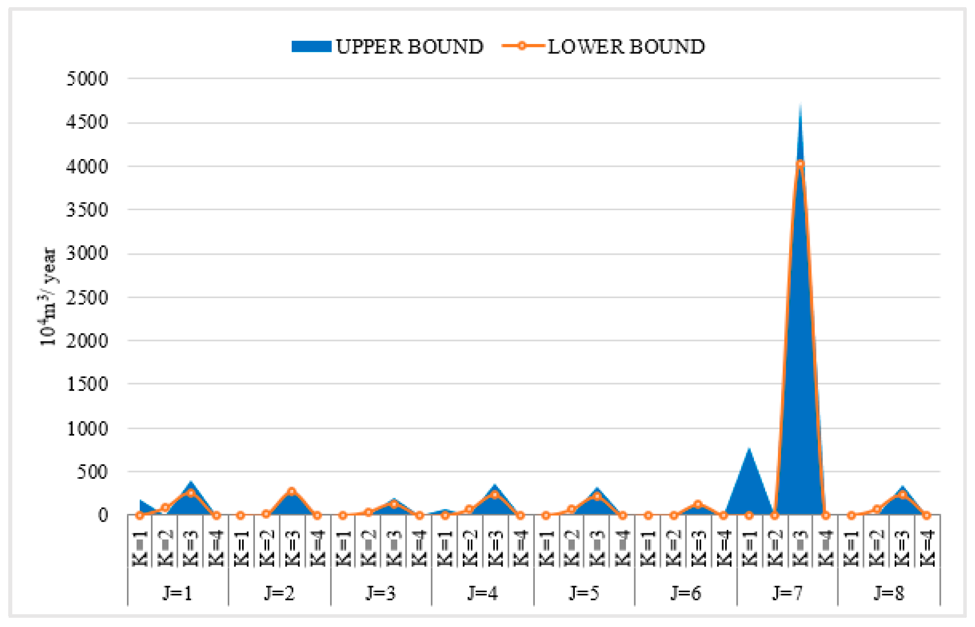
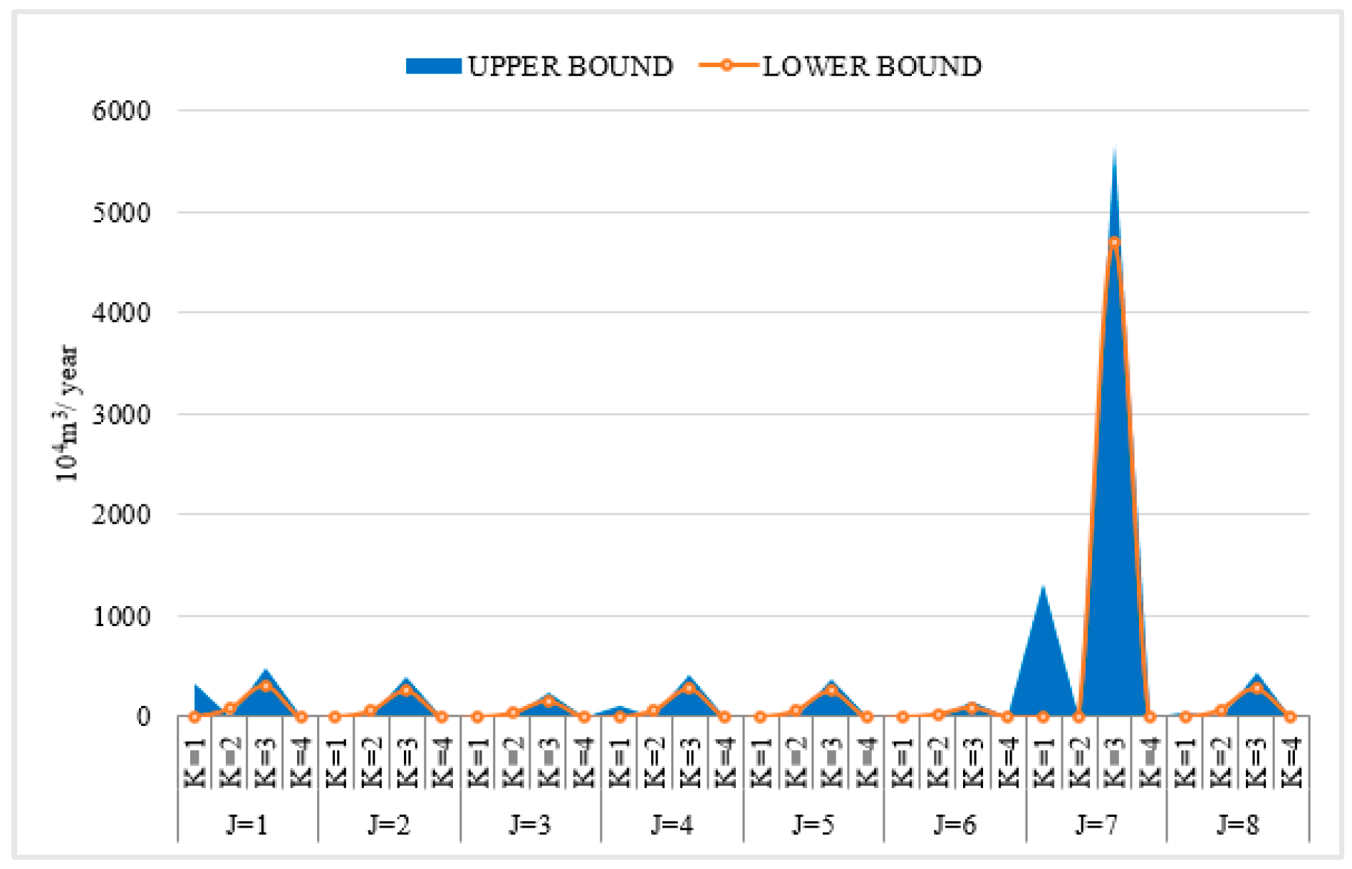
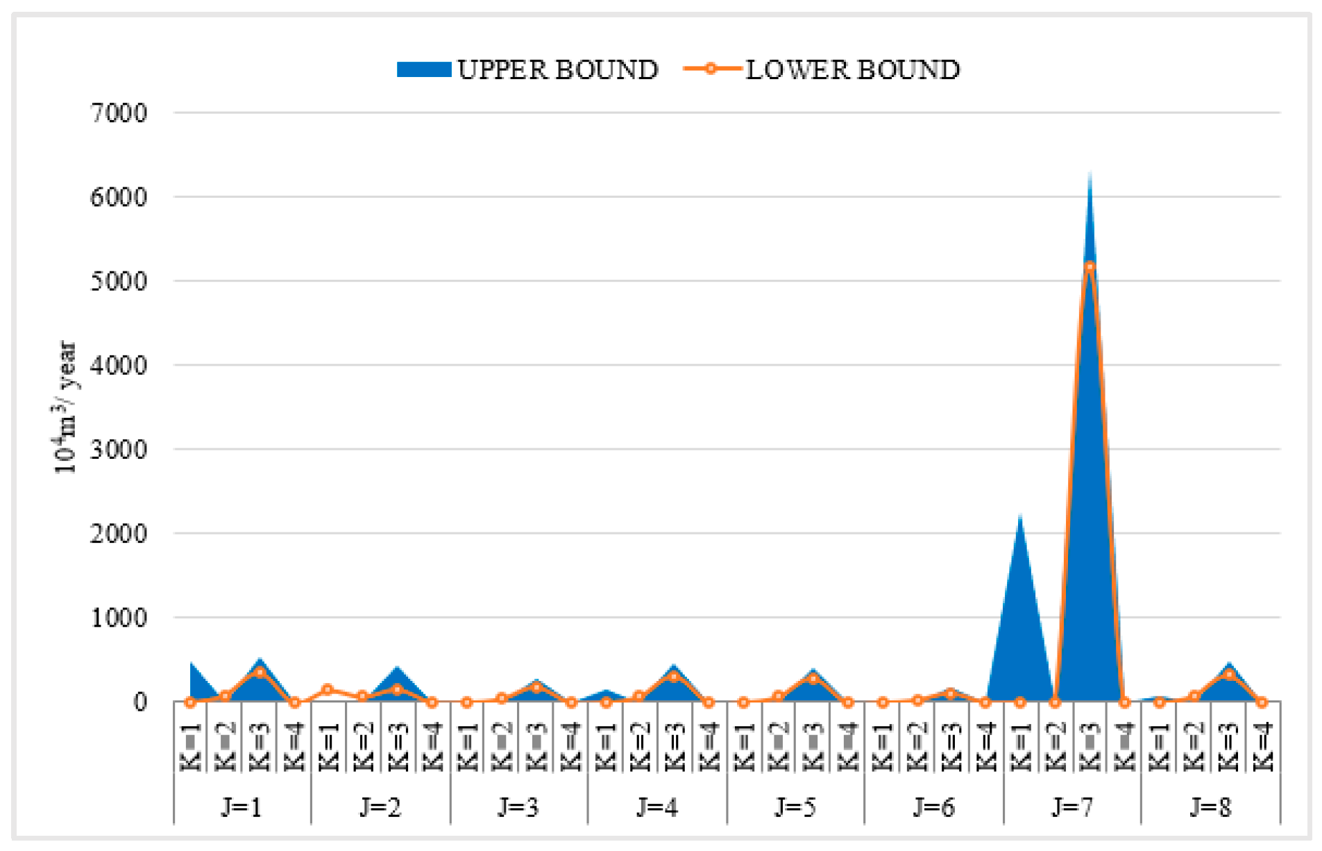
| Areas | Department | T = 1 | T = 2 | T = 3 |
|---|---|---|---|---|
| J = 1 | K = 1 | [184.40, 0.00] | [320.20, 0.00] | [481.64, 481.64] |
| K = 2 | [0.00, 86.25] | [0.00, 86.70] | [0.00, 87.10] | |
| K = 3 | [407.58, 505.71] | [474.42, 664.80] | [527.05, 353.56] | |
| K = 4 | [0.00, 0.00] | [0.00, 0.00] | [0.00, 0.00] | |
| J = 2 | K = 1 | [0.00, 0.00] | [0.00, 0.00] | [0.00, 139.80] |
| K = 2 | [0.00, 13.58] | [0.00, 66.40] | [0.00, 66.65] | |
| K = 3 | [335.60, 267.85] | [393.04, 259.34] | [424.11, 154.04] | |
| K = 4 | [0.00, 0.00] | [0.00, 0.00] | [0.00, 0.00] | |
| J = 3 | K = 1 | [0.00, 0.00] | [0.00, 0.00] | [0.00, 0.00] |
| K = 2 | [0.00, 40.10] | [0.00, 40.60] | [0.00, 41.15] | |
| K = 3 | [208.17, 134.02] | [243.33, 160.29] | [274.24, 182.71] | |
| K = 4 | [0.00, 0.00] | [0.00, 0.00] | [0.00, 0.00] | |
| J = 4 | K = 1 | [67.91, 0.00] | [102.18, 0.00] | [148.20, 0.00] |
| K = 2 | [0.00, 70.10] | [0.00, 70.65] | [0.00, 71.15] | |
| K = 3 | [361.67, 302.19] | [418.25, 381.11] | [466.88, 464.11] | |
| K = 4 | [0.00, 0.00] | [0.00, 0.00] | [0.00, 0.00] | |
| J = 5 | K = 1 | [0.00, 0.00] | [0.00, 0.00] | [0.00, 0.00] |
| K = 2 | [0.00, 64.15] | [0.00, 64.50] | [0.00, 64.80] | |
| K = 3 | [327.70, 214.40] | [386.24, 254.65] | [414.72, 287.71] | |
| K = 4 | [0.00, 0.00] | [0.00, 0.00] | [0.00, 0.00] | |
| J = 6 | K = 1 | [0.00, 0.00] | [0.00, 0.00] | [0.00, 0.00] |
| K = 2 | [0.00, 0.00] | [0.00, 27.55] | [0.00, 27.65] | |
| K = 3 | [124.09, 124.09] | [146.15, 94.90] | [166.04, 110.73] | |
| K = 4 | [0.00, 0.00] | [0.00, 0.00] | [0.00, 0.00] | |
| J = 7 | K = 1 | [784.86, 0.00] | [1216.12, 0.00] | [2118.36, 0.00] |
| K = 2 | [0.00, 0.00] | [0.00, 0.00] | [0.00, 0.00] | |
| K = 3 | [4735.23, 4789.06] | [5672.73, 5640.26] | [6321.98, 6515.96] | |
| K = 4 | [0.00, 0.00] | [0.00, 0.00] | [0.00, 0.00] | |
| J = 8 | K = 1 | [13.81, 0.00] | [243.10, 0.00] | [352.30, 0.00] |
| K = 2 | [0.00, 69.35] | [0.00, 70.55] | [0.00, 71.80] | |
| K = 3 | [354.27, 242.83] | [230.12, 296.91] | [194.17, 338.50] | |
| K = 4 | [0.00, 0.00] | [0.00, 0.00] | [0.00, 0.00] |
| Areas | Pollution | T = 1 | T = 2 | T = 3 |
|---|---|---|---|---|
| J = 1 | R = 1 | [11,331.82, 11,152.21] | [10,198.64, 10,036.99] | [9178.78, 9033.29] |
| R = 2 | [812.42, 799.54] | [731.18, 719.59] | [658.06, 647.63] | |
| J = 2 | R = 1 | [5630.28, 5541.04] | [5067.25, 4986.94] | [4560.53, 4488.24] |
| R = 2 | [495.89, 488.03] | [446.30, 439.23] | [401.67, 395.31] | |
| J = 3 | R = 1 | [9805.01, 9649.60] | [8824.51, 8684.64] | [7942.06, 7816.18] |
| R = 2 | [537.59, 529.07] | [483.83, 476.17] | [435.45, 428.55] | |
| J = 4 | R = 1 | [26,910.25, 23,835.35] | [24,219.22, 21,451.81] | [21,797.30, 19,306.63] |
| R = 2 | [1304.28, 1155.25] | [1173.85, 1039.72] | [1056.47, 935.75] | |
| J = 5 | R = 1 | [34,731.30, 34,180.81] | [31,258.17, 30,762.73] | [28,132.35, 27,686.45] |
| R = 2 | [2128.55, 2094.81] | [1915.69, 1885.33] | [1724.12, 1696.80] | |
| J = 6 | R = 1 | [6601.18, 6496.55] | [5941.06, 5846.90] | [5346.96, 5262.21] |
| R = 2 | [387.63, 381.48] | [348.86, 343.33] | [313.98, 309.00] | |
| J = 7 | R = 1 | [35,123.98, 34,567.27] | [31,611.58, 31,110.54] | [28,450.43, 27,999.49] |
| R = 2 | [5581.30, 5492.83] | [5023.17, 4943.55] | [4520.85, 4449.19] | |
| J = 8 | R = 1 | [32,417.50, 28,713.32] | [29,175.75, 25,841.98] | [26,258.18, 23,257.79] |
| R = 2 | [1666.91, 1476.44] | [1500.22, 1328.80] | [1350.20, 1195.92] |
| Areas | Pollution | Department | H = 1 | H = 2 | H = 3 |
|---|---|---|---|---|---|
| I = 1 | R = 1 | T = 1 | [390.00, 351.00] | [464.10, 414.18] | [543.00, 480.45] |
| T = 2 | [360.00, 324.00] | [428.40, 382.32] | [501.23, 443.49] | ||
| T = 3 | [315.00, 283.50] | [374.85, 334.53] | [438.57, 388.05] | ||
| R = 2 | T = 1 | [19.50, 17.55] | [23.21, 20.71] | [27.15, 24.02] | |
| T = 2 | [18.00, 16.20] | [21.42, 19.12] | [25.06, 22.17] | ||
| T = 3 | [16.50, 14.85] | [19.64, 17.52] | [22.97, 20.33] | ||
| I = 2 | R = 1 | T = 1 | [87.00, 78.30] | [103.53, 92.39] | [121.13, 107.18] |
| T = 2 | [75.00, 67.50] | [89.25, 79.65] | [104.42, 92.39] | ||
| T = 3 | [66.00, 59.40] | [78.54, 70.09] | [91.89, 81.31] | ||
| R = 2 | T = 1 | [7.80, 7.02] | [9.28, 8.28] | [10.86, 9.61] | |
| T = 2 | [7.20, 6.48] | [8.57, 7.65] | [10.02, 8.87] | ||
| T = 3 | [6.90, 6.21] | [8.21, 7.33] | [9.61, 8.50] | ||
| I = 3 | R = 1 | T = 1 | [645.00, 580.50] | [767.55, 684.99] | [898.03, 794.59] |
| T = 2 | [630.00, 567.00] | [749.70, 669.06] | [877.15, 776.11] | ||
| T = 3 | [600.00, 540.00] | [714.00, 637.20] | [835.38, 739.15] | ||
| R = 2 | T = 1 | [37.50, 33.75] | [44.63, 39.83] | [52.21, 46.20] | |
| T = 2 | [36.00, 32.40] | [42.84, 38.23] | [50.12, 44.35] | ||
| T = 3 | [33.00, 29.70] | [39.27, 35.05] | [45.95, 40.65] | ||
| I = 4 | R = 1 | T = 1 | [1305.00, 1174.50] | [1552.95, 1385.91] | [1816.95, 1607.66] |
| T = 2 | [1260.00, 1134.00] | [1499.40, 1338.12] | [1754.30, 1552.22] | ||
| T = 3 | [1215.00, 1093.50] | [1445.85, 1290.33] | [1691.64, 1496.78] | ||
| R = 2 | T = 1 | [73.50, 66.15] | [87.47, 78.06] | [102.33, 90.55] | |
| T = 2 | [70.50, 63.45] | [83.90, 74.87] | [98.16, 86.85] | ||
| T = 3 | [66.00, 59.40] | [78.54, 70.09] | [91.89, 81.31] | ||
| I = 5 | R = 1 | T = 1 | [295.50, 265.95] | [351.65, 313.82] | [411.42, 364.03] |
| T = 2 | [285.00, 256.50] | [339.15, 302.67] | [396.81, 351.10] | ||
| T = 3 | [270.00, 243.00] | [321.30, 286.74] | [375.92, 332.62] | ||
| R = 2 | T = 1 | [19.50, 17.55] | [23.21, 20.71] | [27.15, 24.02] | |
| T = 2 | [18.90, 17.01] | [22.49, 20.07] | [26.31, 23.28] | ||
| T = 3 | [18.00, 16.20] | [21.42, 19.12] | [25.06, 22.17] | ||
| I = 6 | R = 1 | T = 1 | [1830.00, 1647.00] | [2177.70, 1943.46] | [2547.91, 2254.41] |
| T = 2 | [1770.00, 1593.00] | [2106.30, 1879.74] | [2464.37, 2180.50] | ||
| T = 3 | [1680.00 1512.00] | [1999.20, 1784.16] | [2339.06, 2069.63] | ||
| R = 2 | T = 1 | [99.00, 89.10] | [117.81, 105.14] | [137.84, 121.96] | |
| T = 2 | [93.00, 83.70] | [110.67, 98.77] | [129.48, 114.57] | ||
| T = 3 | [85.50, 76.95] | [101.75, 90.80] | [119.04, 105.33] | ||
| I = 7 | R = 1 | T = 1 | [690.00, 621.00] | [821.10, 732.78] | [960.69, 850.02] |
| T = 2 | [660.00, 594.00] | [785.40, 700.92] | [918.92, 813.07] | ||
| T = 3 | [615.00, 553.50] | [731.85, 653.13] | [856.26, 757.63] | ||
| R = 2 | T = 1 | [43.50, 39.15] | [51.77, 46.20] | [60.57, 53.59] | |
| T = 2 | [42.00, 37.80] | [49.98, 44.60] | [58.48, 51.74] | ||
| T = 3 | [39.00, 35.10] | [46.41, 41.42] | [54.30, 48.04] | ||
| I = 8 | R = 1 | T = 1 | [1110.00, 999.00] | [1320.90, 1178.82] | [1545.45, 1367.43] |
| T = 2 | [1005.00, 904.50] | [1195.95, 1067.31] | [1399.26, 1238.08] | ||
| T = 3 | [900.00, 810.00] | [1071.00, 955.80] | [1253.07, 1108.73] | ||
| R = 2 | T = 1 | [57.00, 51.30] | [67.83, 60.53] | [79.36, 70.22] | |
| T = 2 | [51.00, 45.90] | [60.69, 54.16] | [71.01, 62.83] | ||
| T = 3 | [46.50, 41.85] | [55.34, 49.38] | [64.74, 57.28] | ||
| I = 9 | R = 1 | T = 1 | [2610.00, 2349.00] | [3105.90, 2771.82] | [3633.90, 3215.31] |
| T = 2 | [2370.00, 2133.00] | [2820.30, 2516.94] | [3299.75, 2919.65] | ||
| T = 3 | [2130.00, 1917.00] | [2534.70, 2262.06] | [2965.60, 2623.99] | ||
| R = 2 | T = 1 | [135.00, 121.50] | [160.65, 143.37] | [187.96, 166.31] | |
| T = 2 | [124.50, 112.05] | [148.16, 132.22] | [173.34, 153.37] | ||
| T = 3 | [111.00, 99.90] | [132.09, 117.88] | [154.55, 136.74] | ||
| I = 10 | R = 1 | T = 1 | [14,100.00, 12,690.00] | [16,779.00, 14,974.20] | [19,631.43, 17,370.07] |
| T = 2 | [12,750.00, 11,475.00] | [15,172.50, 13,540.50] | [17,751.83, 15,706.98] | ||
| T = 3 | [11,550.00, 10,395.00] | [13,744.50, 12,266.10] | [16,081.07, 14,228.68] | ||
| R = 2 | T = 1 | [705.00, 634.50] | [838.95, 748.71] | [981.57, 868.50] | |
| T = 2 | [630.00, 567.00] | [749.70, 669.06] | [877.15, 776.11] | ||
| T = 3 | [570.00, 513.00] | [678.30, 605.34] | [793.61, 702.19] | ||
| I = 11 | R = 1 | T = 1 | [945.00, 850.50] | [1124.55, 1003.59] | [1315.72, 1164.16] |
| T = 2 | [855.00, 769.50] | [1017.45, 908.01] | [1190.42, 1053.29] | ||
| T = 3 | [780.00, 702.00] | [928.20, 828.36] | [1085.99, 960.90] | ||
| R = 2 | T = 1 | [46.50, 41.85] | [55.34, 49.38] | [64.74, 57.28] | |
| T = 2 | [42.00, 37.80] | [49.98, 44.60] | [58.48, 51.74] | ||
| T = 3 | [37.50, 33.75] | [44.63, 39.83] | [52.21, 46.20] |
| Species | Upper Limit | Lower Limit |
|---|---|---|
| Stabilize the cost of water shortage | 0.00 | 12,673,946.38 |
| Stabilize the use cost of water resources | 0.00 | 20,265.92 |
| Stabilize the cost of sewage treatment | 0.00 | 4414.19 |
3. Results Analysis and Discussion
3.1. Total Pollutant Control in the Yinma River Basin Based on ITSR Optimization Method
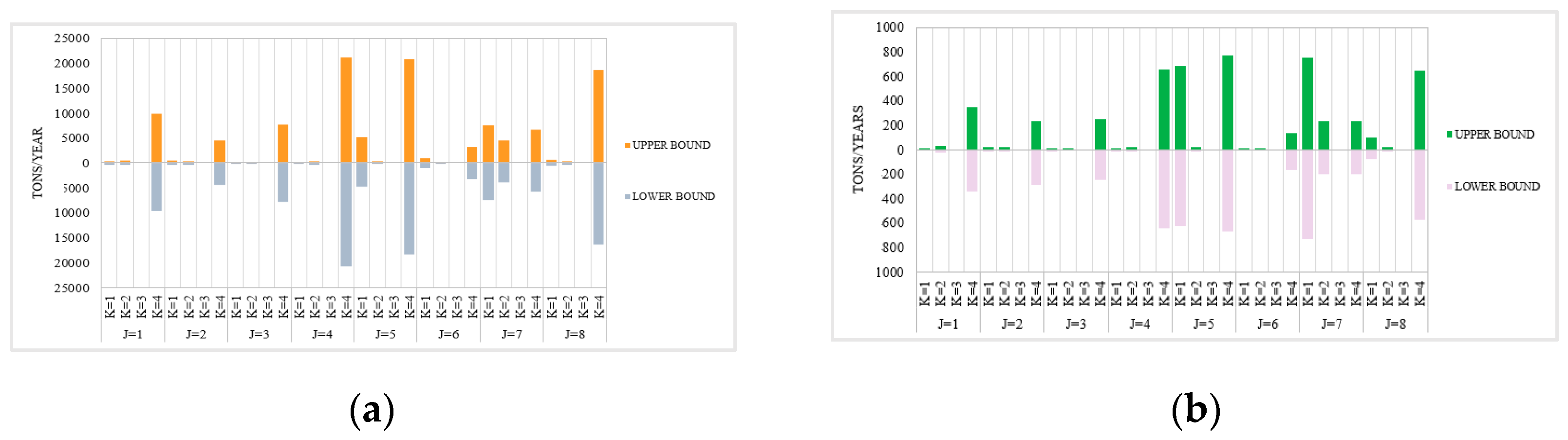
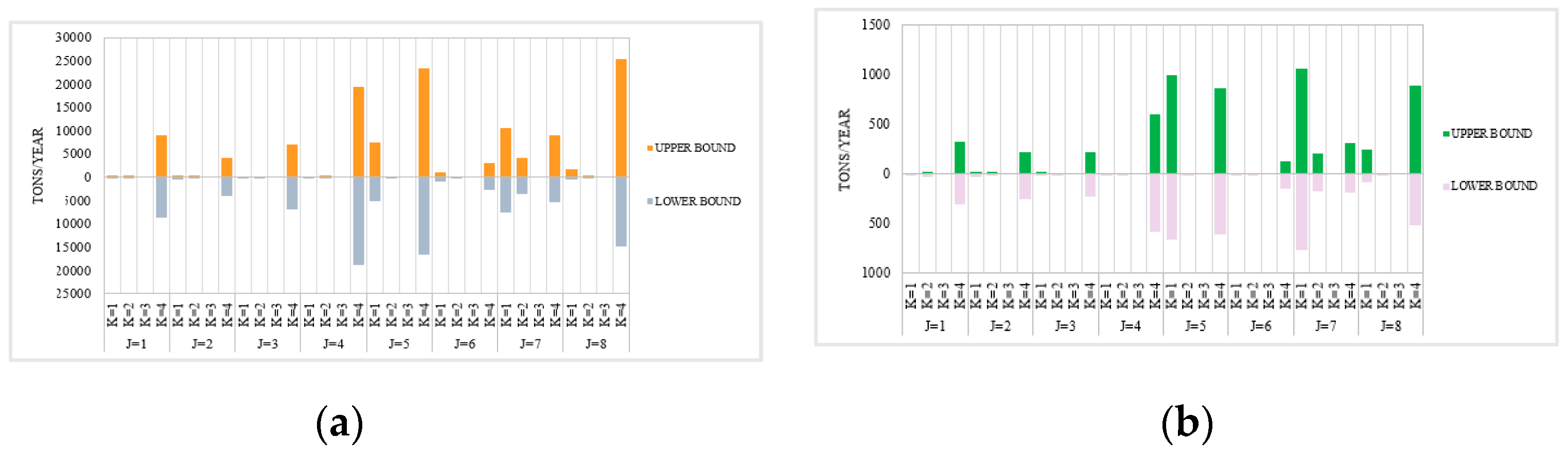
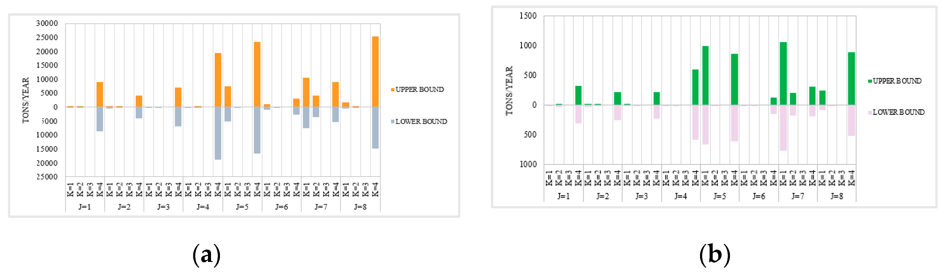
3.1.1. Analysis of the Changes in Sewage Discharge in the Yinma River Basin Based on the ITSR Optimization Method
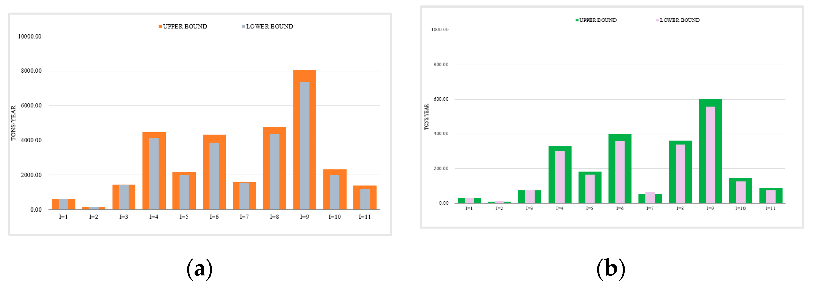
3.1.2. Analysis of the Change of Pollutants Inflow Variation in the Yinma River Basin Based on the ITSR Optimization Method
3.2. Figures, Tables and Schemes
3.3. Analysis the Change of Water Resources Distribution Scheme Based on ITSR Optimization Method
3.3.1. Water Resources Distribution Scheme Based on ITSR Optimization Method
3.3.2. Analysis of the Change of Water Shortage for the Water Uses Departments in Each Planning Area Based on the ITSR Optimization Method
3.3.3. Redistribution of the Used Water in the Different Water Use Departments in Each Planning Area Based on the ITSP Optimization Method
3.4. Scenario Analysis Based on the ITSP Optimization Method
3.4.1. Scenario Analysis Under Low Water Resources Utilization Level in the First Planning Period
3.4.2. Analysis of the Influence of Different Robust Coefficients on the Economic Benefit of the System
4. Conclusions
Author Contributions
Funding
Acknowledgments
Conflicts of Interest
References
- Tan, Z.Y. Study on the Construction of Water Resources use Control system in China. Leg. Syst. Expo 2020, 15, 206–207. [Google Scholar]
- Sharma, P.; Kumar, S.N. The global governance of water, energy, and food nexus: Distribution and access for competing demands. Int. Environ. Agreem.-Politics Law Econ. 2020, 20, 377–391. [Google Scholar] [CrossRef]
- Qu, G.D.; Lou, Z.H. Application of Particle Swarm Algorithm in the Optimal Distribution of Areal Water Researches Based on Immune Evolutionary Algorithm. J. Shanghai Jiaotong Univ. 2013, 18, 634–640. [Google Scholar] [CrossRef]
- Sun, W.; Zeng, Z.J. City Optimal Allocation of Water Resources Research Based on Sustainable Development. Adv. Mater. Res. 2012, 446–449, 2703–2707. [Google Scholar] [CrossRef]
- Hu, Z.N.; Chen, Y.Z.; Yao, L.M.; Wei, C.T.; Li, C.Z. Optimal allocation of regional water resources: From a perspective of equity–efficiency tradeoff. Resour. Conserv. Recycl. 2016, 109, 102–113. [Google Scholar] [CrossRef]
- Wang, S.J.; Hou, Y.; Zhang, X.L.; Ding, J. Progress and Prospect of Research on optimal distribution of Water Resources in China. Water Resour. Dev. Res. 2002, 9, 9–11. [Google Scholar]
- Zhao, B.; Dong, Z.C.; Xu, D. Rational distribution of areal water resources, water supply of different quality and its model. People’s Yangtze River 2004, 2, 21–22. [Google Scholar]
- Guan, J.N.; Wang, J.; Pan, H.; Yang, C.; Qu, J.; Lu, N.; Yuan, X. Heavy metals in Yinma River sediment in a major Phaeozems zone, Northeast China: Distribution, chemical fraction, contamination assessment and source apportionment. Sci. Rep. 2018, 8, 22–31. [Google Scholar] [CrossRef] [Green Version]
- Li, S.J.; Zhang, J.Q.; Guo, E.L.; Zhang, F.; Ma, Q.Y.; Mu, G.Y. Dynamics and ecological risk assessment of chromophoric dissolved organic matter in the Yinma River Watershed: Rivers, reservoirs, and urban waters. Environ. Res. 2017, 158, 245–254. [Google Scholar] [CrossRef]
- Chen, Y.N.; Zhang, J.Q.; Zhang, F.; Liu, X.P.; Zhou, M. Contamination and health risk assessment of PAHs in farmland soils of the Yinma River Basin, China. Ecotoxicol. Environ. Saf. 2018, 156, 383–390. [Google Scholar] [CrossRef]
- Li, C.; Zhou, J.; Ouyang, S. Water Resources Optimal Allocation Based on Large-scale Reservoirs in the Upper Reaches of Yangtze River. Water Resour. Manag. 2015, 29, 2171–2187. [Google Scholar] [CrossRef]
- Chen, B.; Chen, G.Q.; Hao, F.H.; Yang, Z.F. Exergy-based water resource distribution of the mainstream Yellow River. Commun. Nonlinear Sci. Numer. Simul. 2009, 14, 1721–1728. [Google Scholar] [CrossRef]
- Abdulbaki, D.; Al-Hindi, M.; Yassine, A.; Najm, M.A. An optimization model for the distribution of water resources. J. Clean. Prod. 2017, 164, 994–1006. [Google Scholar] [CrossRef]
- Song, W.Z.; Yuan, Y.; Jiang, Y.Z.; Lei, X.H.; Shu, D.C. Rule-based water resource distribution in the Central Guizhou Province, China. Ecol. Eng. 2016, 87, 192–202. [Google Scholar] [CrossRef]
- Di, H.; Liu, X.P.; Zhang, J.Q.; Tong, Z.J.; Ji, M.C. The Spatial Distributions and Variations of Water Environmental Risk in Yinma River Basin, China. Int. J. Environ. Res. Public Health 2018, 15, 521. [Google Scholar] [CrossRef] [Green Version]
- Meng, C.; Wang, X.; Li, Y. An Optimization Model for Water Management Based on Water Resources and Environmental Carrying Capacity: Case Study of the Yinma River Basin, Northeast China. Water 2018, 10, 65. [Google Scholar] [CrossRef] [Green Version]
- Huang, J.R. Research on Algorithm and Applications of Robust Optimization. Ph.D. Thesis, Xi’an University of Technology, Xi’an, China, 2012. [Google Scholar]
- Chen, J.; Koebis, E.; Yao, J.C. Optimality Conditions and Duality for Robust Nonsmooth Multiobjective Optimization Problems with Restrictions. J. Optim. Theory Appl. 2019, 181, 411–436. [Google Scholar] [CrossRef]
- Minoux, M. On 2-stage robust LP with RHS uncertainty: Complexity results and applications. J. Glob. Optim. 2011, 49, 521–537. [Google Scholar] [CrossRef]
- Zheng, T. A robust methodology for design optimizations of electromagnetic devices under uncertainties. Int. J. Appl. Electromagn. Mech. 2019, 59, 71–78. [Google Scholar] [CrossRef]
- Imbens, G.W.; Kolesár, M. Robust standard errors in small samples: Some practical advice. Rev. Econ. Stat. 2016, 98, 701–712. [Google Scholar] [CrossRef]
- Guo, Z.S.; Li, Y. An interval robust stochastic programming method for planning carbon sink trading to support areal ecosystem sustainability-a case study of Zhangjiakou, China. Ecol. Eng. 2017, 104, 99–115. [Google Scholar] [CrossRef]
- Tan, Y.; Cao, Y.J.; Li, C.B.; Li, Y.; Zhou, J.J.; Song, Y. A two-stage stochastic programming approach considering risk level for distribution network soperation with wind power. IEEE Syst. J. 2016, 10, 117. [Google Scholar] [CrossRef]
- Kammammettu, S.; Li, Z.K. Two-Stage Robust Optimization of Water Treatment Network Design and Operations under Uncertainty. Ind. Eng. Chem. Res. 2020, 59, 1218–1233. [Google Scholar] [CrossRef]
- Qiu, Y.; Liu, Y.; Liu, Y.; Chen, Y.Z.; Li, Y. An Interval Two-stage Stochastic Programming Model for Flood Resources Distribution under Ecological Benefits as a Restriction Combined with Ecological Compensation Concept. Int. J. Environ. Res. Public Health 2019, 16, 1033. [Google Scholar] [CrossRef] [PubMed] [Green Version]
- Natarajan, K.; Pachamanova, D.; Sim, M. Incorporating Asymmetric Distributional Information in Robust Value-at-Risk Optimization. Manag. Sci. 2008, 14, 626. [Google Scholar] [CrossRef] [Green Version]
- Zhang, F.; Liu, X.P.; Zhang, J.Q.; Wu, R.N.; Ma, Q.Y.; Chen, Y.N. Ecological vulnerability assessment based on multi-sources data and SD model in Yinma River Basin, China. Ecol. Model. 2017, 349, 41–50. [Google Scholar] [CrossRef]
- Wang, F.L. Study on Rational Distribution of Areal Water Resources. Ph.D. Thesis, Wuhan University of Technology, Wuhan, China, 2013. [Google Scholar]
- Liu, N.L.; Jiang, H.Q.; Wu, W.J. Empirical research of optimal distribution model of water resources under uncertainties. China Environ. Sci. 2014, 3, 1607–1613. [Google Scholar]


| Areas | Interval-Two-Stage | Interval-Two-Stage-Robust | ||||||
|---|---|---|---|---|---|---|---|---|
| Industrial | Municipal | Ecological | Agriculture | Industrial | Municipal | Ecological | Agriculture | |
| J = 1 | [574, 910] | [1380, 2083] | [396, 498] | [20.727, 26.334] | [573, 758] | [1380, 1736] | [396, 498] | [20,727, 21,945] |
| J = 2 | [168, 266] | [1058, 1609] | [304, 383] | [8939, 11.358] | [222, 222] | [1111, 1341] | [304, 383] | [8939, 9465] |
| J = 3 | [731, 926] | [642, 978] | [182, 229] | [9116, 11.384] | [772, 772] | [642, 815] | [182, 229] | [9116, 9487] |
| J = 4 | [1366, 2167] | [1122, 1699] | [326, 410] | [26.298, 33.028] | [1738, 1806] | [1122, 1416] | [326, 410] | [26.298, 27.523] |
| J = 5 | [4475, 5678] | [1026, 1565] | [300, 377] | [45.819, 57 545] | [4475, 4732] | [1026, 1283] | [300, 377] | [45.819, 45.819] |
| J = 6 | [538, 684] | [438, 664] | [126, 157] | [12.696, 16 243] | [538, 538] | [641, 553] | [126, 157] | [12.696, 13,536] |
| J = 7 | [9114, 14,440] | [16,685, 22,583] | [4410, 5524] | [11.272, 14.158] | [10.378, 12.033] | [16.685, 18.539] | [5081, 5524] | [11.272, 11.272.00] |
| J = 8 | [1036, 1549] | [1110, 1691] | [319, 401] | [61.958, 77.813] | [1173, 1291] | [1110, 1387] | [319, 401] | [61.958, 61.958] |
| Areas | Interval-Two-Stage | Interval-Two-Stage-Robust | ||||||
|---|---|---|---|---|---|---|---|---|
| Industrial | Municipal | Ecological | Agriculture | Industrial | Municipal | Ecological | Agriculture | |
| J = 1 | [0.00, 0.00] | [345.00, 746.66] | [426.00, 195.94] | [0.00, 0.00] | [0.00, 0.00] | [0.00, 0.00] | [0.00, 0.00] | [0.00, 0.00] |
| J = 2 | [0.00, 0.00] | [470.01, 583.49] | [343.68, 345.67] | [0.00, 0.00] | [0.00, 0.00] | [0.00, 0.00] | [0.00, 0.00] | [0.00, 0.00] |
| J = 3 | [0.00, 0.00] | [160.40, 221.72] | [0.00, 213.62] | [5914.80, 6826.40] | [0.00, 0.00] | [0.00, 0.00] | [0.00, 0.00] | [0.00, 0.00] |
| J = 4 | [0.00, 0.00] | [280.40, 430.68] | [0.00, 357.59] | [17,248.80, 19,878.60] | [0.00, 0.00] | [0.00, 0.00] | [0.00, 0.00] | [0.00, 0.00] |
| J = 5 | [440.00, 2037.71] | [256.60, 459.05] | [0.00, 262.04] | [30,053.40, 34,635.30] | [1052.85, 1614.34] | [0.00, 0.00] | [0.00, 0.00] | [13,745.70, 18,237.60] |
| J = 6 | [16.76, 16.76] | [225.20, 259.63] | [129.58, 134.45] | [0.00, 0.00] | [94.94, 94.94] | [0.00, 0.00] | [0.00, 0.00] | [12,696, 13,536] |
| J = 7 | [0.00, 0.00] | [3707.80, 5014.09] | [0.00, 349.83] | [7394.40, 8521.60] | [261.64, 1420.25] | [0.00, 926.95] | [0.00, 0.00] | [3381.60, 4508.80] |
| J = 8 | [0.00, 0.00] | [277.40, 405.21] | [365.21, 364.47] | [13,038.89, 46,833.80] | [460.40, 830.60] | [0.00, 0.00] | [0.00, 0.00] | [18,587.40, 24,783.20] |
| Areas | Interval-Two-Stage | Interval-Two-Stage-Robust | ||||||
|---|---|---|---|---|---|---|---|---|
| Industrial | Municipal | Ecological | Agriculture | Industrial | Municipal | Ecological | Agriculture | |
| J = 1 | [0.00, 0.00] | [0.00, 746.66] | [0.00, 195.94] | [0.00, 0.00] | [0.00, 0.00] | [0.00, 0.00] | [0.00, 0.00] | [0.00, 0.00] |
| J = 2 | [0.00, 0.00] | [00.00, 583.49] | [0.00, 345.67] | [0.00, 0.00] | [0.00, 0.00] | [0.00, 0.00] | [0.00, 0.00] | [0.00, 0.00] |
| J = 3 | [0.00, 0.00] | [0.00, 221.72] | [0.00, 00.00] | [0.00, 6826.40] | [0.00, 0.00] | [0.00, 0.00] | [0.00, 0.00] | [0.00, 0.00] |
| J = 4 | [0.00, 0.00] | [0.00, 430.68] | [0.00, 0.00] | [0.00, 9049.65] | [0.00, 0.00] | [0.00, 0.00] | [0.00, 0.00] | [0.00, 0.00] |
| J = 5 | [0.00, 1049.51] | [0.00, 459.05] | [0.00, 0.00] | [0.00, 0.00] | [480.60, 1126.42] | [0.00, 0.00] | [0.00, 0.00] | [13,745.70, 18,237.60] |
| J = 6 | [16.76, 16.76] | [0.00, 259.63] | [0.00, 134.45] | [0.00, 0.00] | [94.94, 94.94] | [0.00, 0.00] | [0.00, 0.00] | [0.00, 0.00] |
| J = 7 | [0.00, 0.00] | [0.00, 5014.09] | [0.00, 0.00] | [0.00, 8521.60] | [0.00, 153.75] | [0.00, 926.95] | [0.00, 0.00] | [3381.60, 4508.80] |
| J = 8 | [0.00, 0.00] | [0.00, 405.21] | [0.00, 0.00] | [0.00, 46,833.80] | [0.00, 830.60] | [0.00, 0.00] | [0.00, 0.00] | [0.00, 24,783.20] |
| Areas | Interval-Two-Stage | Interval-Two-Stage-Robust | ||||||
|---|---|---|---|---|---|---|---|---|
| Industrial | Municipal | Ecological | Agriculture | Industrial | Municipal | Ecological | Agriculture | |
| J = 1 | [0.00, 0.00] | [0.00, 0.00] | [0.00, 0.00] | [0.00, 0.00] | [0.00, 0.00] | [0.00, 0.00] | [0.00, 0.00] | [0.00, 0.00] |
| J = 2 | [0.00, 0.00] | [0.00, 0.00] | [0.00, 0.00] | [0.00, 0.00] | [0.00, 0.00] | [0.00, 0.00] | [0.00, 0.00] | [0.00, 0.00] |
| J = 3 | [0.00, 0.00] | [0.00, 0.00] | [0.00, 0.00] | [0.00, 0.00] | [0.00, 0.00] | [0.00, 0.00] | [0.00, 0.00] | [0.00, 0.00] |
| J = 4 | [0.00, 0.00] | [0.00, 0.00] | [0.00, 0.00] | [0.00, 0.00] | [0.00, 0.00] | [0.00, 0.00] | [0.00, 0.00] | [0.00, 0.00] |
| J = 5 | [0.00, 13.00] | [0.00, 459.05] | [0.00, 0.00] | [0.00, 0.00] | [0.00, 614.65] | [0.00, 0.00] | [0.00, 0.00] | [12,542.66, 18,237.60] |
| J = 6 | [16.76, 16.76] | [0.00, 0.00] | [0.00, 0.00] | [0.00, 0.00] | [94.94, 94.94] | [0.00, 0.00] | [0.00, 0.00] | [0.00, 0.00] |
| J = 7 | [0.00, 0.00] | [0.00, 0.00] | [0.00, 0.00] | [0.00, 0.00] | [0.00, 0.00] | [0.00, 926.95] | [0.00, 0.00] | [0.00, 4508.80] |
| J = 8 | [0.00, 0.00] | [0.00, 0.00] | [0.00, 0.00] | [0.00, 0.00] | [0.00, 0.00] | [0.00, 0.00] | [0.00, 0.00] | [0.00, 11,608.56] |
| Areas | Interval-Two-Stage | Interval-Two-Stage-Robust | ||||||
|---|---|---|---|---|---|---|---|---|
| Industrial | Municipal | Ecological | Agriculture | Industrial | Municipal | Ecological | Agriculture | |
| Panshi | 0.00 | 545.83 | 310.97 | 0.00 | 0.00 | 0.00 | 0.00 | 0.00 |
| Yongji | 0.00 | 526.75 | 344.68 | 0.00 | 0.00 | 0.00 | 0.00 | 0.00 |
| Shuangyang | 0.00 | 191.06 | 106.81 | 6370.60 | 0.00 | 0.00 | 0.00 | 0.00 |
| Jiutai | 0.00 | 355.54 | 178.80 | 18,563.70 | 0.00 | 0.00 | 0.00 | 0.00 |
| Dehui | 1238.86 | 357.83 | 131.02 | 32,344.35 | 1333.60 | 0.00 | 0.00 | 16,036.65 |
| Yitong | 16.76 | 242.42 | 132.02 | 0.00 | 94.94 | 44.22 | 0.00 | 0.00 |
| Changchun | 0.00 | 4360.95 | 174.92 | 7958.00 | 840.94 | 463.48 | 0.00 | 3945.20 |
| Nongan | 0.00 | 341.31 | 364.84 | 29,936.35 | 645.50 | 0.00 | 0.00 | 21,685.30 |
Publisher’s Note: MDPI stays neutral with regard to jurisdictional claims in published maps and institutional affiliations. |
© 2020 by the authors. Licensee MDPI, Basel, Switzerland. This article is an open access article distributed under the terms and conditions of the Creative Commons Attribution (CC BY) license (http://creativecommons.org/licenses/by/4.0/).
Share and Cite
He, W.; Yang, L.; Li, M.; Meng, C.; Li, Y. Application of an Interval Two-Stage Robust (ITSR) Optimization Model for Optimization of Water Resource Distribution in the Yinma River Basin, Jilin Province, China. Water 2020, 12, 2910. https://doi.org/10.3390/w12102910
He W, Yang L, Li M, Meng C, Li Y. Application of an Interval Two-Stage Robust (ITSR) Optimization Model for Optimization of Water Resource Distribution in the Yinma River Basin, Jilin Province, China. Water. 2020; 12(10):2910. https://doi.org/10.3390/w12102910
Chicago/Turabian StyleHe, Wei, Luze Yang, Minghao Li, Chong Meng, and Yu Li. 2020. "Application of an Interval Two-Stage Robust (ITSR) Optimization Model for Optimization of Water Resource Distribution in the Yinma River Basin, Jilin Province, China" Water 12, no. 10: 2910. https://doi.org/10.3390/w12102910