Modelling of the Complex Groundwater Level Dynamics during Episodic Rainfall Events of a Surficial Aquifer in Southern Italy

Abstract

We analyzed the complex dynamics that are involved the groundwater level variations due to the episodic rainfall supply in the Ionian coastal plain surficial aquifer located in Southern Italy. In this aquifer, as a consequence of the particular hydrogeological framework, both direct and lateral recharge mechanisms coexist. Hence, the dynamics of groundwater level variations are quite complex and strongly non-linear. Our focus was essentially on the short-term behavior of groundwater levels, with a specific analysis on episodic rainfall events. To model these dynamics, due to the presence of the preferential pathways in the infiltration processes, a kinematic dispersion wave model was used. Specifically, a one-dimensional and non-linear particle-based numerical model was developed. It uses ideal particles with constant water volume travel, according to celerity and hydraulic dispersion, to simulate the infiltration rate wave through the vadose zone. The infiltration rate that reaches the water table represents the input function to evaluate the aquifer groundwater level fluctuations. As a consequence of the special lithological and storage capacity characteristics of the surficial layers, groundwater flow conditions change from unconfined to confined. The developed model analyzes the direct groundwater supply under natural conditions, including episodic rainfall, and it has been validated using a high-resolution time series of rainfall data and groundwater level obtained from the monitoring station Terra Montonata.

1. Introduction

To understand and model the relation between groundwater level fluctuations and rainfall events is fundamental to realizing the groundwater supply mechanisms, in order to achieve sustainable management of groundwater resources. In shallow aquifers, where the water table responds quite quickly to rainfall inputs, recharge events may be isolated and associated with individual precipitation events [1,2]. This paper concerns the groundwater-level dynamics in the Ionian coastal plain surficial aquifer in Southern Italy [3,4], where in consequence of the particular hydrogeological framework, both direct and lateral recharge mechanisms coexist. Therefore, the aquifer is characterized by a complex response of groundwater level rises due to episodic rainfall events. It is strongly non-linear and severely dependent by the groundwater level antecedent to the rainfall event. The focus is essentially on the short-term behavior of groundwater level, with a specific analysis on episodic rainfall events framing it in the general hydrogeological context of the area.

On the basis of groundwater level and precipitation time series of sufficient duration and temporal resolution, it is possible to evaluate the influences of rainfall characteristics on episodic groundwater recharge in different hydrogeological conditions and in consequence of different hydro-meteorological events. It is also possible to estimate aquifer parameters, evapotranspiration and effective infiltration from precipitation [5,6].

Short lags between precipitation and groundwater level variations are representative of preferential flow pathways conditioning the supply mechanism in shallow aquifers. Preferential flow in natural soils and rocks under saturated [7,8,9] and unsaturated [10,11,12] conditions is ubiquitous. From the textural point of view, the macropores governing preferential flow dynamics [13,14,15,16] normally have three physically distinct processes: macropore flow, finger flow and funnel flow [17].

The kinematic diffusion wave theory is a useful approach with which to model the vertical movement of infiltrated water under uniform and/or preferential flow [18]. Some authors derived a kinematic diffusion form of the Richards’ equation, mathematically equivalent to the advection diffusion equation [19,20]. Alternative approaches based on Newton’s law found a power law relationship between the infiltration rate and mobile water content [21]. The combination of this functional relationship and the continuity equation gives rise to the kinematic wave model [22]. The latter model assumes that mobile water moves as a film along the preferential pathways in unsaturated porous media, under atmospheric pressure. When that happens, unsaturated flow is only gravity driven and counter balanced by the dissipative friction due to the viscous force, whereas the capillary force is neglected. Experimental evidence [23,24] shows a dispersion effect that attenuates the kinematic wave. Water dispersion phenomena are due to several factors linked to the contributions of mesopores, wherein capillary force may be significant and intricate pore paths are present. Water infiltrates with velocities both greater and less than the mean vertical downward velocity. The introduction of the dispersion component give rise to the kinematic dispersion wave model [25]. The implementation of preferential flow into the numerical model and the evaluation of the model parameters remain the subject of discussion [26].

The modeling of the infiltration processes through the vadose zone and the quantification of the aquifer supply hydrograph are strictly related to the basic hydrogeological characteristics of unsaturated and saturated zones and the surface–subsurface interaction [27].

The assessment of groundwater recharge requires a numerical model able to represent the whole process controlling the infiltration dynamics with a small computational cost. Several authors developed an efficient numerical solution to solve the Richards’ equation for simulating unsaturated flow in layered and heterogeneous porous media [28,29,30].

In this paper a modeling framework with the relative numerical approach is proposed to describe the complex dynamics of infiltration processes during episodic rainfall events and the relative groundwater level variations. The infiltration processes are modelled like a one-dimensional flow along vertical direction using the kinematic dispersion wave model. The governing equations are generally numerically solved by means of Eulerian methods [25]. They normally suffer from numerical problems, such as numerical dispersion and computational complexity, especially as a consequence of severe variations of boundary conditions. During intense rainfall events, the infiltration rate, the water content and the water table fluctuation change rapidly, giving rise to numerical instabilities in the Eulerian numerical model. In order to overcome these difficulties a non-linear particle-based model has been developed to numerically solve the kinematic dispersion wave equation. Particles move according to convection and dispersion terms which are functions of the particle density linked to the mobile water content. Through this particle-based model, the infiltration rate hydrograph of the water table is obtained and it is used to simulate the groundwater fluctuations according to the storage coefficient of the surficial aquifer. The length of the vadose zone changes on the basis of the water table depth.

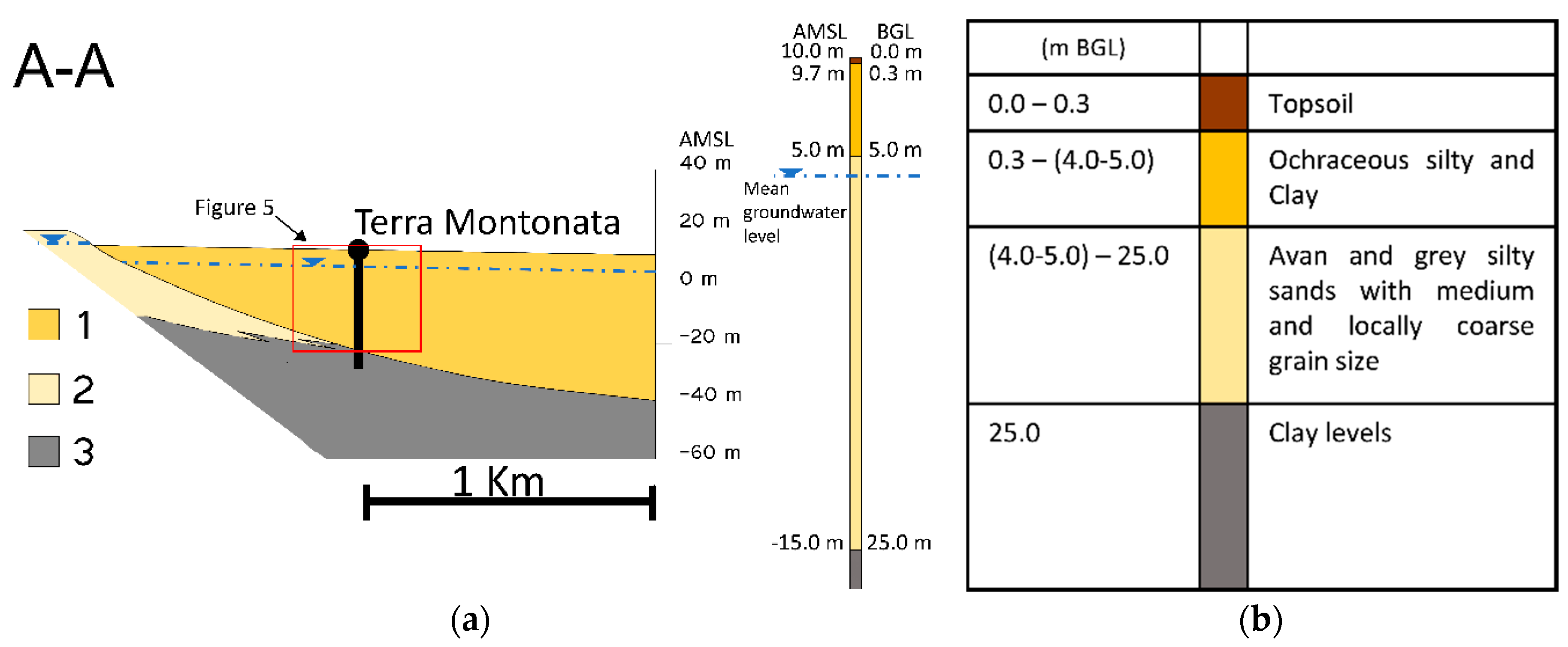
The developed method was applied to the case study of the surficial level of the Ionian coastal plain aquifer. Previous studies carried out on the same aquifer, on the basis of monthly average precipitation and groundwater levels, show that recharge takes place mainly laterally from the upward aquifer, whereas direct recharge is essentially interdicted by the presence of a surficial silty and clay layer [3,4]. The analysis of precipitation and groundwater records at higher resolution scale evidences a quick response to intense rainfall events that are not coherent only with lateral or upward recharge supply. This implies the presence of direct recharge due to the presence of preferential groundwater supply flow-paths crossing the surficial silt and clay layer [31]. In this area, these preferential flow path supplies have been recognized mainly in the several reclamation channels crossing the coastal plain which cut the surficial impervious layer. Moreover, the medium groundwater level is quite close to the stratigraphic transition between the surficial thin silty clayey layer and the sands hosting groundwater. Thus, according to the lithological features of the aquifer, unconfined–confined flow conversion may occur as a consequence of the groundwater level variations, giving rise to a change in the aquifer storage. Hydrogeological parameters have been estimated by comparing modeled results and observed data.

The specific goals of this paper are:

• Improving the understanding of the hydrogeological behavior of the Ionian coastal plain aquifer, highlighting how the geological and lithological features are interrelated with hydrogeologic processes.
• Demonstrating the presence of unconfined–confined flow conditions in the study area.
• Testing whether the kinematic dispersion wave model can adequately represent the infiltration processes due to episodic recharge events in the study area.

2. Materials

2.1. Geological, Lithological and Hydrogeological Setting

The study site is located in a wide and flat area called the Ionian (Metaponto) coastal plain [32]. Its highest elevation is 15 m, facing the Ionian Sea in the southern part of Basilicata region (Southern Italy). In particular, the studied site is within the interfluvial area between Cavone and Basento rivers (Figure 1). Geologically, it is located in the southern part of the Bradanic Trough [33], which is a tectonic trough filled up by a thick sequence of Pliocene to Pleistocene marine sequences, mainly of sub-Apennines clays [30], passing upwards to coarse-grained coastal and continental deposits known as regressive terraced deposits of the Bradanic Through [34]. Immediately upward from the study area are the terraced deposits of the lower order outcropping.

Metaponto plain is characterized by a thick stratigraphic sequence of alluvial, transitional, coastal and marine deposits—described in detail by several authors in [32,33,34,35]. The complex sequence can be simplified as:

(a)

A substratum of middle-late Pleistocene and silty clays of the sub-Apenine type (Argille Subappennine); a formation with an irregular upper boundary at a depth of about 15–30 m, deepening locally in correspondence of the paleovalley.

(b)

Upper unit (late Pleistocene and Holocene) of fluvial and/or deltaic sandy-gravelly deposits with clayey intercalations with a thickness of 15–30 m, deepening locally in accordance with the paleovalley. The plain is covered by a thin layer (4–5 m) of alluvial silty clayey deposits.

The lithological features of the area gave rise to the presence of two main aquifers: the former is hosted in the marine terraces where groundwater flows generally in unconfined conditions in the coarse grained deposits of the terraces; the latter is a coastal aquifer hosted in the sandy coastal plain deposits where the shallowest permeable layer is characterized by free piezometric oscillations. Figure 2a shows the schematic geological cross -section of the area. Figure 2b shows the strata sequence detected in a borehole close to Terra Montonata groundwater monitoring station in the coastal aquifer. The shallowest permeable layer does not outcrop due to the widespread presence of the upper almost impervious stratum, 2 up to 5 m thick constituted by silty clays. Test analyses conducted in the whole Metaponto coastal plain show saturated hydraulic conductivity values in the range 3.47 × 10^–6–5.69 × 10⁻³ ms⁻¹ [3]. Specifically, in the interfluvial area between Cavone and Basento rivers corresponding to the Terra Montonata monitoring station, the hydraulic conductivity has the average value of 2.28 × 10⁻⁴ ms⁻¹.

2.2. General Hydrodynamic Observations

Groundwater dynamics in the present work are analyzed on the basis of time series data collected by Protezione Civile Basilicata—Centro Funzionale Decentrato (http://centrofunzionalebasilicata.it/it/), which has a network of climatic and hydrodynamic stations in the whole Basilicata Region. The data of the monitoring station of Terra Montonata (N = 40°18′17″; E = 16°45′10″; Z = 10 m AMSL) have been considered representative of the hydrological and hydrogeological conditions of the interfluvial area between Basento and Cavone rivers of the coastal plain. Continuous time series of groundwater level and precipitation for a period of ten years (2002–2012) with a time resolution of 20 min have been considered.

Monthly trends in the period 2002–2012 of the rainfall P (mm) and averaged groundwater level Z_w (m AMSL) have been investigated (Figure 3). P presents Mediterranean characteristics with a peak in December and the minimum in August with the average annual precipitation (in 2002–2012 period) equal to 530 mm.

Z_w shows a seasonal behavior characterized by a constant increase in the water level during the autumn and winter period with a peak at the beginning of the spring and a recession period during the spring/summer period.

2.2.1. Lateral/Upward Groundwater Supply

An estimation of groundwater wave propagation from the terraced deposits to the monitoring station is used to demonstrate the presence of the lateral/upward groundwater supply. Saturated groundwater flow in the surficial aquifer can be represented as a one-dimensional flow along the horizontal direction:

$$S\frac{\partial H}{\partial t}=-T\frac{{\partial }^{2}H}{\partial x^2}$$

(1)

where T (LT⁻²) is the transmissivity of aquifer, x is the horizontal direction and S (-) is the storage coefficient. The terraced deposits present a minimum distance from the monitoring station equal to x₀ = 1200 m. The surficial aquifer is characterized by an average hydraulic conductivity value of K = 2.2 × 10⁻⁴ ms⁻¹ with an average thickness of 20 m (Figure 2). Then the transmissivity will be equal to T = 4.4 × 10⁻³ m²s⁻¹. Assuming that the surficial aquifer is subject to an instantaneous unit rise pulse in correspondence with the terraced deposits (x = 0), groundwater level wave will be propagated according to the following analytical solution for the one-dimensional diffusion equation along semi-infinite boundary [36]:

$$H\left(x_0,t\right)=\frac{1}{\sqrt{4\pi D{t}^3}}{x}_{0}exp\left(-\frac{x_0^2}{4Dt}\right)$$

(2)

where $D=T/S$ (LT⁻²) is the hydraulic diffusivity. Equation (2) reaches its peak at time t_p equal to:

$$t_p=\frac{x_0^2}{6D}$$

(3)

This time can be viewed as the time necessary so that a groundwater rise at x = 0 (terraces deposits) leads to the maximum rise at the distance x₀ where the monitoring station of Terra Montonata is located. t_p assumes a value of 121.83 d for S = 0.2, which is a value of S in good agreement with the sandy lithology of the aquifer. This time is coherent with the time lag from the comparison between the average monthly rainfall regime P and the average monthly groundwater level Z_w, which shows 3–4 months as the lag.

2.2.2. Evidence of Direct Groundwater Supply

Even if the main groundwater supply of the aquifer is related to water coming from the terraced deposits, there is also evidence of a quick response of groundwater level to rainfall. Figure 4 shows the comparison between the daily average groundwater level, monthly average groundwater level and daily precipitation for four daily time series during the wet season (1th October–30th April). The analysis of precipitation and groundwater level on a daily time scale evidences the presence of an impulsive response to intense rainfall characterized by an average time lag of 2–3 days. The water table responds immediately to intense rainfall events. This implies there are quite short paths of direct recharge along the vadose zone that contribute to groundwater supply. This behavior is evident from the autumn to spring period, wherein the most significant rainfall events in terms of intensity, magnitude and amount of precipitation occur.

Long term lateral recharge combines with direct recharge that takes place along the vadose zone. As shown in Figure 4, the daily groundwater level falling after rising due to significant rainfall events decreases exponentially according to the following recursive expression [37]:

$$Z_w^{i+1}=Z_w^0+\left(Z_w^i-Z_w^0\right)exp\left(\frac{t^i-t^{i+1}}{\tau }\right)$$

(4)

where $Z_w^0$ (L) is the groundwater level that would be attained if no direct recharge occurred, $Z_w^{i+1}$ (L) is the groundwater level at time $t^{i+1}$, $Z_w^i$ (L) is the groundwater level at time $t^i$ and $\tau$ (T) is the recession time. Recession time assumes a value of 18 days, whereas $Z_w^0$ changes significantly depending on lateral/upward groundwater recharge mechanism.

Moreover, as shown in Figure 4, the surficial aquifer presents a different hydraulic behavior during the rainfall event depending on the initial value of the groundwater level antecedent to the episodic rainfall events. This behavior seems to be interrelated to the depth of the bed of the surficial silty and clay unit (gray bar on Figure 4). If groundwater level is below the bottom of the silty clay stratum, the unconfined condition eventuates; otherwise, the aquifer becomes confined and the storage property of surficial aquifer decreases. Then groundwater level increases.

3. Methods

3.1. Rainfall Infiltration Dynamics

The key observations described in the previous sections led us to establish the conceptual model of the infiltration processes in the vadose zone and groundwater recharge highlighted in Figure 5. The studied area of the coastal plain is largely covered by arable crops with topsoil more or less 0.30 m deep. Given that the investigated period regards only the cold season, the evapotranspiration processes are negligible. Thus, they have not been taken into account. Below the topsoil, the thin silty and clay layer is present. The permeability characteristics of this layer are not consistent with the observed quick responses of the groundwater levels due to the episodic rainfall events. Thus, they have to be attributed to a preferential flow infiltration mechanism in the vadose zone.

Preferential flow occurs under various conditions at different spatial and temporal scales. In the study area there are several reclamation channels that represent local surface depressions dug up to 2–3 m and more from the soil surface, where surficial flow may concentrate and transmit to the underlying the surficial aquifer. Moreover, hydromechanic processes at larger scale are the consequence also of macropore dynamics related to shrinkage cracks formed by drying of swelling phenomena and by earthworm biopores. Earthworms present a diameter of 1–3 mm and can extend up to 6 m in vertical length. Shrinkage cracks give rise to a rapid movement of depth of around 1 m and more [38]. As a consequence, water accumulates, backfilling the void space.

In the Darcian scale preferential flow mechanisms can be due to unstable flow. Under certain conditions, the wetting front moving downwards breaks into fingers. They represent preferential pathways that facilitate recharge flow. Compression of air below the wetting front causes instability [39] and the wetting front breakup into fingers.

When the precipitation p(t) (LT⁻¹) exceeds the infiltration capacity of the topsoil q_c (LT⁻¹), runoff surficial flow is generated, increasing the infiltration rate in the top soil q(0, t) (LT⁻¹) along the preferential flow paths. Moreover, the infiltration rate of topsoil is limited according to the following expression:

$$q\left(0,t\right)=min\left(q_{crit},p\left(t\right)\right)$$

(5)

where q_crit (LT⁻¹) represents the critical value of the infiltration rate. The precipitation in excess does not feed the preferential flow paths [40]. The infiltration travels along the vadose zone, reaching the water table, giving rise to the infiltration rate hydrograph at water table q(L, t) (LT⁻¹). L (L) is the water table depth from topsoil.

3.2. Groundwater-Level Variation Analysis

The raising of the groundwater level is governed by q(L, t) and the storage coefficient S (-). The total rate of the ground water level fluctuation during the episodic recharge is the sum of the recession and accretion rate:

$$\frac{dH}{dt}=\frac{q\left(L,t\right)}{S\left(L\right)}-\frac{H\left(t\right)}{\tau }$$

(6)

where H (L) is the height of the groundwater level above the base level $Z_w^0$, $dH/dt$ (LT⁻¹) is the total change rate of the groundwater level, q(L, t)/S(L) is the accretion rate and $H\left(t\right)/\tau$ is the recession rate. Due to the expected groundwater flow conversion mechanism, S is represented as function of the water table depth L.

In order to investigate the groundwater level fluctuation processes, starting from the time series on an hourly time scale, several rainfall events have been isolated. Each event has been analyzed individually, determining an estimation of the average storage coefficient $\overline{S}$ and the time lag $\Delta t_m$ between the infiltration rate in the topsoil and the accretion rate. They represent two key parameters that characterize the groundwater fluctuation dynamics during the episodic recharge events.

First, for each isolated episodic rainfall event, the cumulative accretion rate function can be determined using the follow recursive equation derived by Equation (6):

$${\displaystyle \sum }_{i=1}^j{\left(\frac{q\left(L,t\right)}{S\left(L\right)}\right)}_i={\displaystyle \sum }_{i=1}^j\left(\frac{H_i}{\tau }+\frac{H_i-H_{i-1}}{\Delta t}\right)i\le j=1\dots .,n$$

(7)

Then, the average value of storage coefficient $\overline{S}$ can be determined as the ratio between the total infiltration in the topsoil and the total accretion:

$$\overline{S}=\frac{{\sum }_{i=1}^{n}q{\left(0,t\right)}_i}{{\sum }_{i=1}^n{\left(\frac{q\left(L,t\right)}{S\left(L\right)}\right)}_i}$$

(8)

The infiltration rate for the topsoil q(0, t) is a function of the precipitation p(t) and the parameters q_c and q_crit. According to the permeability of the surficial thin clayey matrix of the topsoil, q_c has been assumed to be equal to 0.5 mmh⁻¹.

The parameter q_crit governs the susceptibility of the preferential flow in the study area. It represents the maximum infiltration rate which can travel along the preferential flow paths in the vadose zone. According to Equations (5) and (8) the average storage coefficient $\overline{S}$ increases as q_crit increases. Besides, the values of $\overline{S}$ must be consistent with the value of the storage coefficient equal to 0.2, which is coherent with a time lag of 3–4 months between the average monthly rainfall regime and the average monthly groundwater level, as discussed in the previous section. Then, q_crit has been estimated to be equal to 6 mmh⁻¹, which allows one to have the value for the average storage coefficients $\overline{S}$ (determined for each rainfall event) closest to 0.2.

Successively, for each event, the time lag between the cumulative infiltration rate at the water table and the cumulative accretion rate, as the difference between the respective residence times, has been estimated:

$$\Delta t_m={\displaystyle \sum }_{j=1}^n\left(1-\frac{{\sum }_{i=1}^j{\left(q/S\right)}_i}{{\sum }_{i=1}^n{\left(q/S\right)}_i}\right)-{\displaystyle \sum }_{j=1}^n\left(1-\frac{{\sum }_{i=1}^{j}q{\left(0,t\right)}_i}{{\sum }_{i=1}^{n}q{\left(0,t\right)}_i}\right)$$

(9)

Table 1. Analysis of significant episodic rainfall events.

N	Date Interval (month/day/year)	Total Precipitation (mm)	Total Infiltration (mm)	Total Accretion (m)	Average GWL (m)	Average Storage (-)	Time Lag (day)
1	11/01/02–01/04/03	277.80	222.60	1.43	5.48	0.16	9.11
2	01/04/03–02/28/03	127.60	91.00	1.33	5.28	0.07	2.97
3	12/01/03–12/20/03	163.60	97.20	0.68	4.97	0.14	2.19
4	12/20/03–01/18/04	52.20	38.30	0.50	5.24	0.08	3.84
5	11/01/04–11/25/04	216.80	114.40	0.83	4.88	0.14	2.79
6	11/26/04–01/12/05	87.60	68.60	1.06	5.17	0.06	2.69
7	12/01/05–12/26/05	102.40	76.80	0.51	4.65	0.15	2.83
8	02/15/06–03/06/06	83.20	63.10	0.58	4.69	0.11	2.56

illustrates, for each isolated episodic rainfall event, characterized by the value of the total precipitation, the estimated value of the total infiltration rate, the total accretion, the average groundwater level (GWL), the average storage and the time lag.

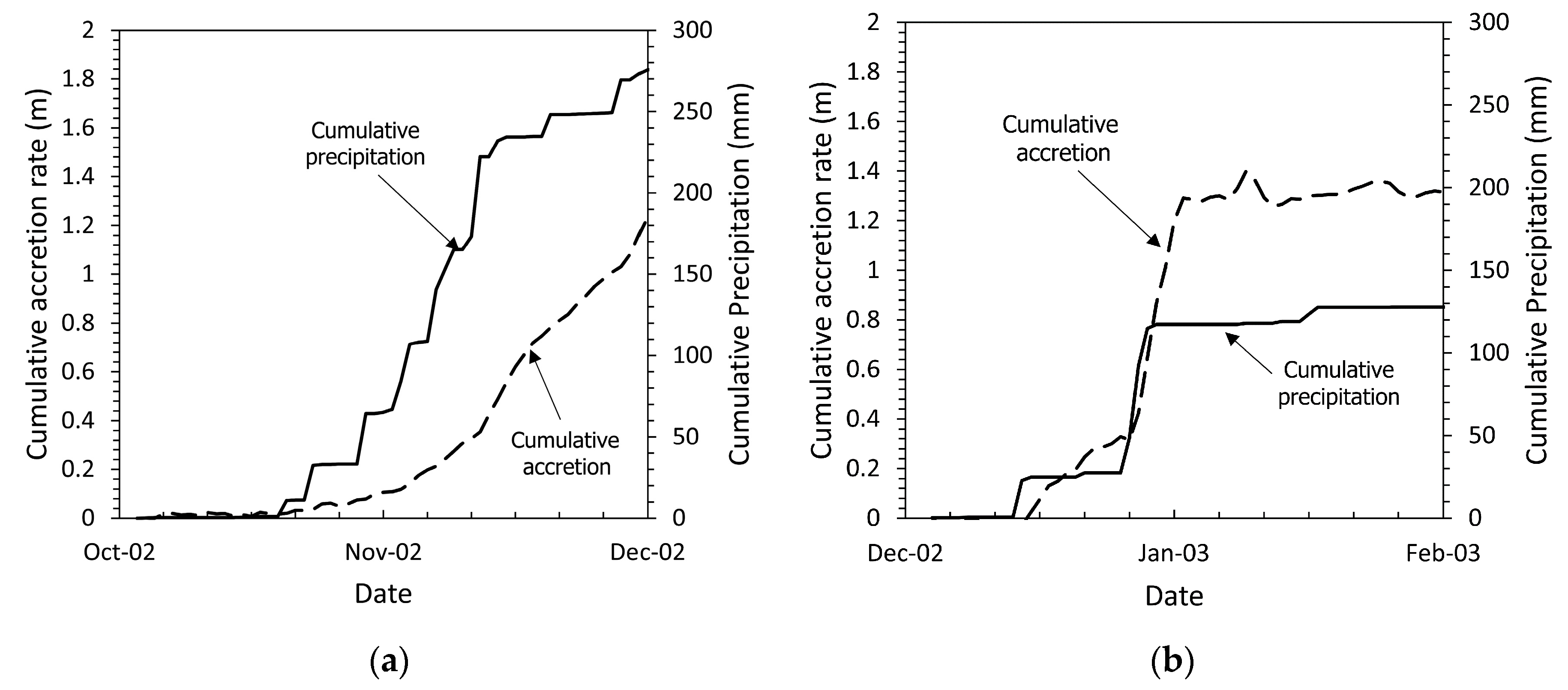
Figure 6 shows the comparison between the cumulative precipitation and the cumulative accretion for event #1 and event #2. The cumulative precipitation in event #1 increases more smoothly. Event #2 is characterized by a time lag higher than event #1. Moreover, Figure 6 highlights a fundamental aspect of the episodic recharge behavior in the study area. The cumulative accretion increases systematically when the groundwater level exceeds the bottom of the silty clay unit (≈5.0 m AMSL). As shown in Table 1, $\overline{S}$ decreases, reaching a value of 0.07 for the event #2, 0.08 for event #4 and 0.06 for the event #6. For events characterized by a groundwater peak below the bottom of the impervious layer, the storage parameter reaches a value in the range 0.11–0.16. 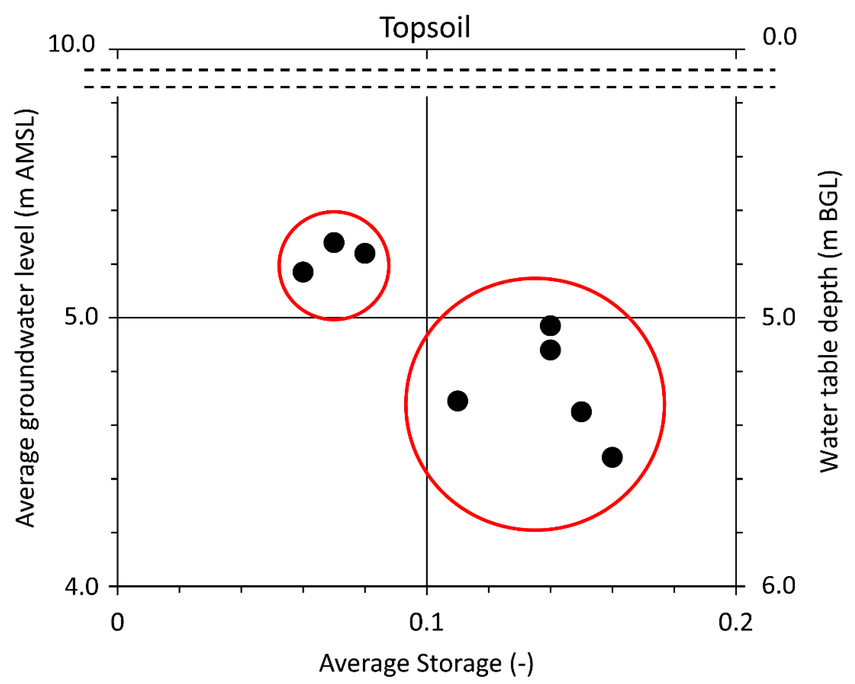Figure 7 shows $\overline{S}$ as a function of the average groundwater level. $\overline{S}$ is systematically lower than 0.10 when the average groundwater level is above ≈ 5.0 m AMSL.

The calculated lag times confirm the presence of a direct recharge mechanism in the study area through preferential pathways. They vary in the range between 2.19 and 9.11 day.

3.3. Kinematic Dispersion Wave Model

The kinematic dispersion wave model is used to represent the preferential infiltration processes along the vadose zone and to determine the infiltration rate hydrograph at water table. Details on the kinematic dispersion wave model can be found in [25]. For convenience, a brief introduction for this approach has been reported. Fluid flow through the one-dimensional variably unsaturated medium occurs through preferential pathways; no exchange exists between the impervious stratum and the preferential pathway. Assuming water density as constant and neglecting the inertial terms in the momentum equation, the conservation laws can be written as:

$$\frac{\partial \theta \left(z,t\right)}{\partial t}+\frac{\partial q\left(z,t\right)}{\partial z}=0$$

(10)

$$q\left(z,t\right)=b{\left[\theta \left(z,t\right)\right]}^a+{\alpha }_w\frac{\partial \theta \left(z,t\right)}{\partial t}$$

(11)

where θ (L³L⁻³) is the mobile volumetric water content within a volume V (L³) of soil profile flowing along preferential pathways, b (LT⁻¹) is the conductance term, a is the preferential flow distribution index, α_w (L) is the water dispersivity coefficient. Starting from the conservation laws, [25] derived a non-linear kinematic dispersion wave equation to describe infiltration processes with the infiltration rate q as the state variable:

$$\frac{\partial q\left(z,t\right)}{\partial t}+c_w\left(\theta \left(z,t\right)\right)\frac{\partial q\left(z,t\right)}{\partial z}=D_w\left(\theta \left(z,t\right)\right)\frac{{\partial }^{2}q\left(z,t\right)}{\partial z^2}$$

(12)

where $D_w$ (L²T⁻¹) is the hydraulic dispersion and $c_w$ (LT⁻¹) is the celerity.

The infiltration rate wave propagates through convection and dispersion processes governed by the changes of the mobile volumetric water content along the preferential pathways. According to [25], celerity is defined as the derivative of the infiltration rate respect to the mobile volumetric water content under $\partial \theta /\partial t$ constant:

$$c_w={\frac{\partial q}{\partial \theta }|}_{\frac{\partial \theta }{\partial t}=const}$$

(13)

whereas hydraulic dispersion depends on the celerity and the water dispersivity coefficient:

$$D_w={\alpha }_w{c}_w$$

(14)

Celerity can be written as:

$$c_w={\frac{\partial q}{\partial \theta }|}_{\frac{\partial \theta }{\partial t}=const}\Rightarrow c_w=ab{\theta }^{a-1}$$

(15)

By combining Equation (15) with Equation (11), the following expression of celerity as a function of the infiltration rate is obtained:

$$c_w=a{b}^{\frac{1}{a}}{q}^{\frac{a-1}{a}}$$

(16)

The infiltration processes depend on three parameters a, b and α_w. The following initial and boundary conditions have been imposed:

$$q\left(z,t\right)=q_0 z>0, t=0$$

(17)

$$q\left(z,t\right)=q\left(0,t\right) z=0, t>0$$

(18)

Equation (12) has been solved numerically using non-linear random walk method. The numerical scheme is described in the following section. The program was written in Matlab.

3.4. Numerical Model

The random-walk method uses particle tracking to solve kinematic process, whereas dispersion processes are simulated by adding random displacement to each particle in addition to advective displacement. It is known that the space-time distribution of particles can be represented by the Fokker–Planck equation, which is not identical to Equation (12). In analogy to the solute transport problem, the celerity term c_w is replaced by:

$${c_w}^{’}=c_w+\frac{\partial D_w}{\partial z}$$

(19)

For each time step Δt, the specific volume of water which enters the subsoil at z = 0 is $w_{in}=q\left(0,t\right) \times \Delta t$ (L). The accumulated specific water volume W (L) will be updated as $W_{t+\Delta t}=W_t+w_{in}$. At z = 0 the flux is strictly convective, so the volumetric water content θ(0, t) will be equal to:

$$\theta \left(0,t\right)={\left(\frac{q\left(0,t\right)}{b}\right)}^{\frac{1}{a}}$$

(20)

N particles each having a specific water volume $\theta \left(0,t\right)/N$ are released at z = 0. The depth z_i of each i-th particle at time t + Δt is updated as:

$$z_i\left(t+\Delta t\right)=z_i\left(t\right)+{c_{w,i}}^{’}\Delta t+Z\sqrt{2D_{w,i}\Delta t}$$

(21)

where Z is a normally distributed random number; c_w,i’ and D_w,i represent the celerity and the hydraulic dispersion associated with the i-th particle. They are functions of the infiltration rate which changes throughout the depth.

The one-dimensional domain along the depth between the topsoil and the water table of length L is discretized with n cells. The infiltration rate and the volumetric water content are assumed constant in space within each cell.

For each cell j (j = 1, …, n) the specific volumetric water content is determined as:

$${\theta }_j^{t+\Delta t}=\frac{n{p}_j^{t+\Delta t}}{{\sum }_{j=1}^{n}n{p}_j^{t+\Delta t}}\frac{W_{t+\Delta t}}{\Delta z}$$

(22)

where np_j is the number of particles within the j-th cell and Δz (L) is the cell size. Once one knows θ_j^t+Δt, the value of the infiltration rate for each cell is determined as:

$$q_j^{t+\Delta t}=b{\left({\theta }_j^{t+\Delta t}\right)}^a+{\alpha }_w\frac{{\theta }_j^{t+\Delta t}-{\theta }_j^t}{\Delta t}$$

(23)

For each particle i, celerity $c_{w,i}$ and hydraulic dispersion $D_{w,i}$ are updated according to the value of the infiltration rate determined in correspondence with the depth z_i.

The specific water volume that reaches the water table is determined on the basis of the number of particles np_out outside the domain (z_i(t + Δt) > L(t)):

$$w_{out}=\frac{n{p}_{out}}{{\sum }_{j=1}^{n}n{p}_j^{t+\Delta t}}{W}_{t+\Delta t}$$

(24)

The infiltration rate that reaches the water table q(t + Δt, L) is determined as:

$$q\left(t+\Delta t,L\left(t\right)\right)=\frac{w_{out}}{\Delta t}$$

(25)

The groundwater level fluctuation is determined using the recursive form of Equation (6):

$$H_{t+\Delta t}=H_{t}exp\left(-\frac{\Delta t}{\tau }\right)+\frac{q\left(t+\Delta t,L\left(t\right)\right)}{S\left(L\left(t\right)\right)}\tau \left(1-exp\left(-\frac{\Delta t}{\tau }\right)\right)$$

(26)

Finally, the domain length L is updated:

$$L\left(t+\Delta t\right)=L\left(0\right)-H_{t+\Delta t}$$

(27)

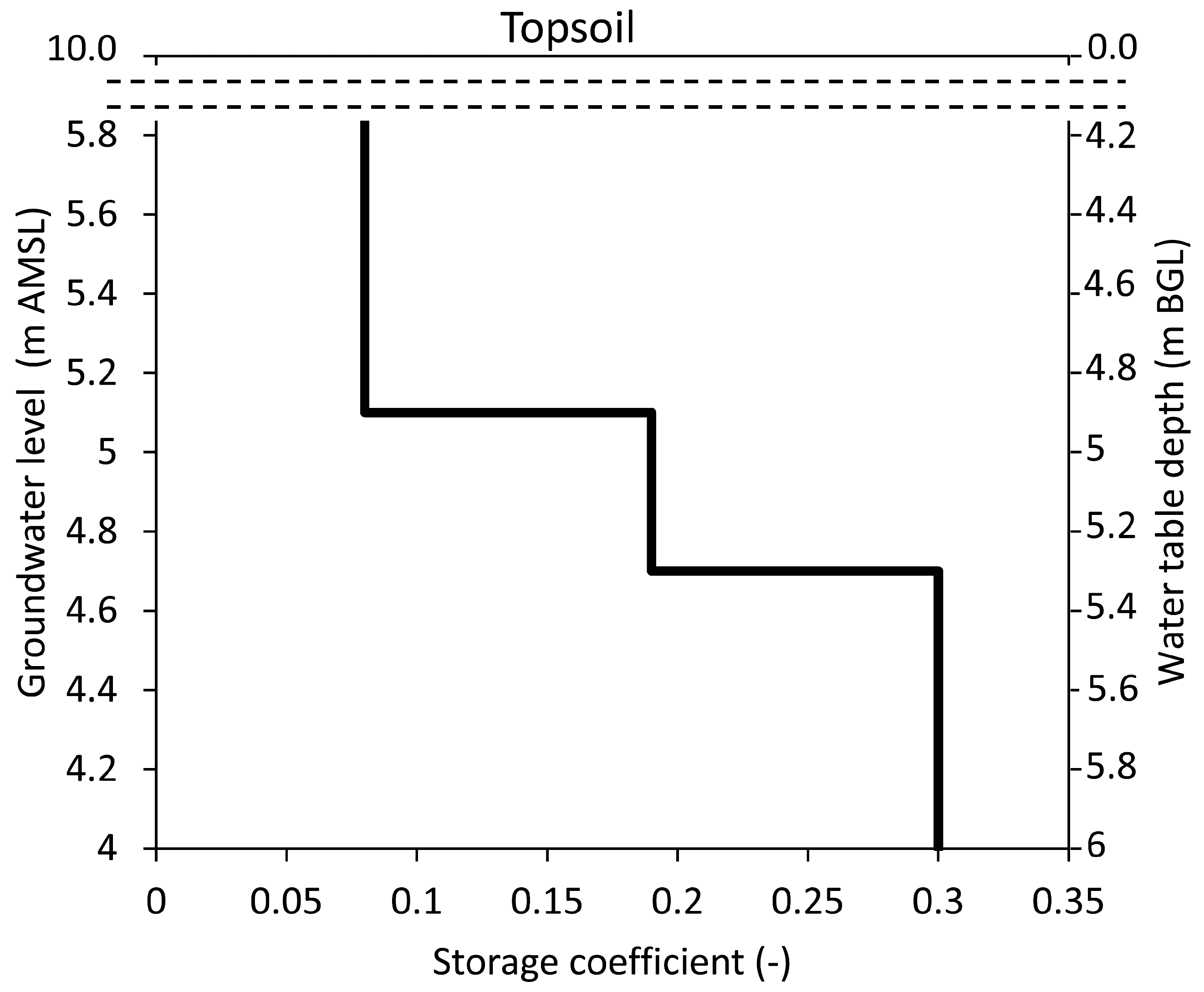
The storage coefficient S changes according to the water table depth L. In particular, having as reference the bottom of the surficial silty clay unit (L₀ = 5 m), two depths have been defined: L₁ = L₀ + d₁ and L₂ = L₀ − d₂. Then S will be equal to: S₁ if the water table depth is higher than L₁; S₂ if the water table depth is lower than L₂; S₀ if the water table depth is between L₁ and L₂.

4. Results

4.1. Simulation Results

The kinematic dispersion model has been used to predict groundwater level fluctuation starting from the hourly precipitation time series. Simulation results have been compared with the observed groundwater level time series. The kinematic dispersion equation has been solved using the developed particle-based model in order to determine the infiltration rate hydrograph at the water table q(L,t). Then groundwater level fluctuation H(t) has been obtained. 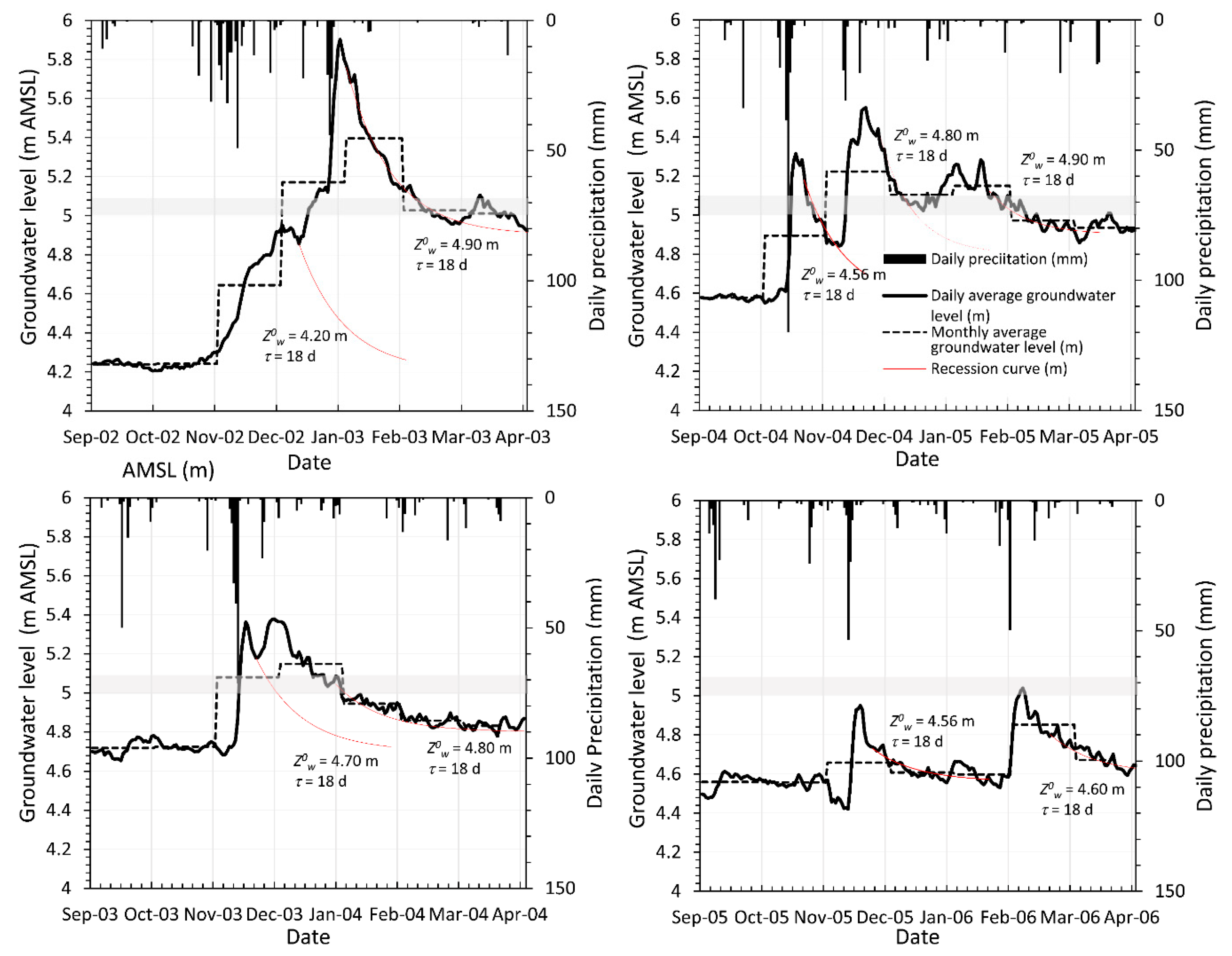Finally, the simulated groundwater level was determined as the sum of H(t) and the value of groundwater level in absence of direct groundwater recharge Z⁰_w. Note that due to the presence of a long-term lateral groundwater recharge mechanism Z⁰_w varies over time, as shown in Figure 4, whereas the recession time τ is constant and equal to 18 day. Simulations began after summer. Thus, the initial mobile water content and the infiltration rate were set to zero.

In order to control the efficiency and performance of the simulation, the time step Δt and the grid cell size Δz for the evaluation of the particle density were chosen so as to satisfy a small Courant number C_o < 0.1. For each time step, a number of particles equal to 10⁵ × [q(0, t + Δt)/b]^1/a were released in the top soil. The time of the simulation was equal to 212 d, corresponding to a period between October 1st and April 30th. According to kinematic theory [21] the parameter a assumes a value equal to either 2 or 3. α_w and b have been estimated by means of the comparison between the observed groundwater levels and the simulated ones.

The parameters involved in the proposed infiltration model have been estimated by the minimization of the root mean square error (RMSE) between the observed groundwater level time series and simulated ones:

$$RMSE=\sqrt{{\left(Z_w^{*}\left(t\right)-Z_w\left(t\right)\right)}^2}$$

(28)

where $Z_w^{*}\left(t\right)$ and $Z_w\left(t\right)$ are the observed and simulated groundwater levels, respectively. The Levenberg–Marquardt algorithm has been used to minimize Equation (28). The optimized values are b = 3.6 × 10⁴ mmh⁻¹ for a = 3 and 3.6 × 10³ mmh⁻¹ for a = 2 and α_w = 200 mm.

Figure 8 shows the estimated step function of the storage coefficient. It decreases as the groundwater level increases, reaching a value lower than 0.1 when the groundwater level is higher than ≈5 m AMSL.

To highlight the strong linear behavior of the groundwater level variations due to the episodic rainfall events, a parametric analysis of the storage coefficient has been done. Further simulations have been conducted using the optimized values of a, b and α_w, while imposing a constant value of the storage coefficient instead of the step function shown in Figure 8.

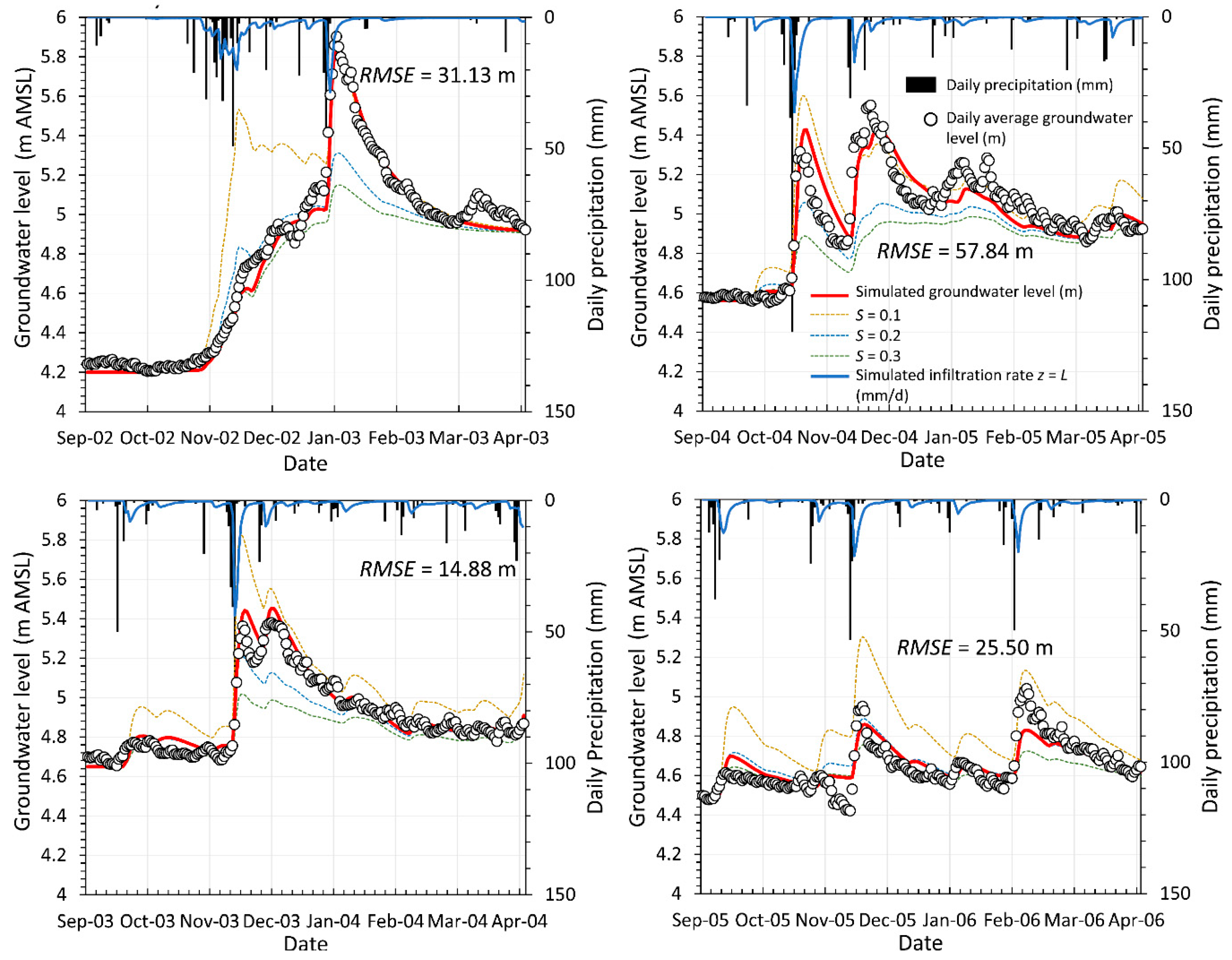
The fitting results are shown in Figure 9. Moreover, the figure highlights the simulated groundwater level that would be attained with a constant value of the storage coefficient.

The infiltration model shows a satisfactory fitting predicting the trend of the groundwater level fluctuation with relative accuracy for both rising and falling periods.

The storage coefficient plays an important role in the amplitude of the groundwater level’s rise. When the storage coefficient is assumed as constant, the simulations fail to reproduce the observed groundwater level variations in terms of amplitude. This feature is very evident on the time period 2002–2003. When the groundwater level is lower than ≈5 m AMSL, the model with S = 0.1 overestimates the groundwater level’s rise. Besides, the model with S = 0.2 fits adequately the observed groundwater level rise until it becomes lower than ≈5 m AMSL. The model results are consistent with the stratigraphy detected close to the Terra Montonata monitoring station. The surficial silty and clay unit works as an aquitard, confining locally the surficial aquifer when the groundwater level exceeds the bottom of the surficial silty and clay unit.

The amplitude of the groundwater level rise is governed by the critical infiltration rate also. As shown in the time periods November–December 2003 and October–November 2004, in order to fit the observed data, the critical infiltration rate must limit the precipitation according to Equation (5).

4.2. Analysis of Infiltration Processes

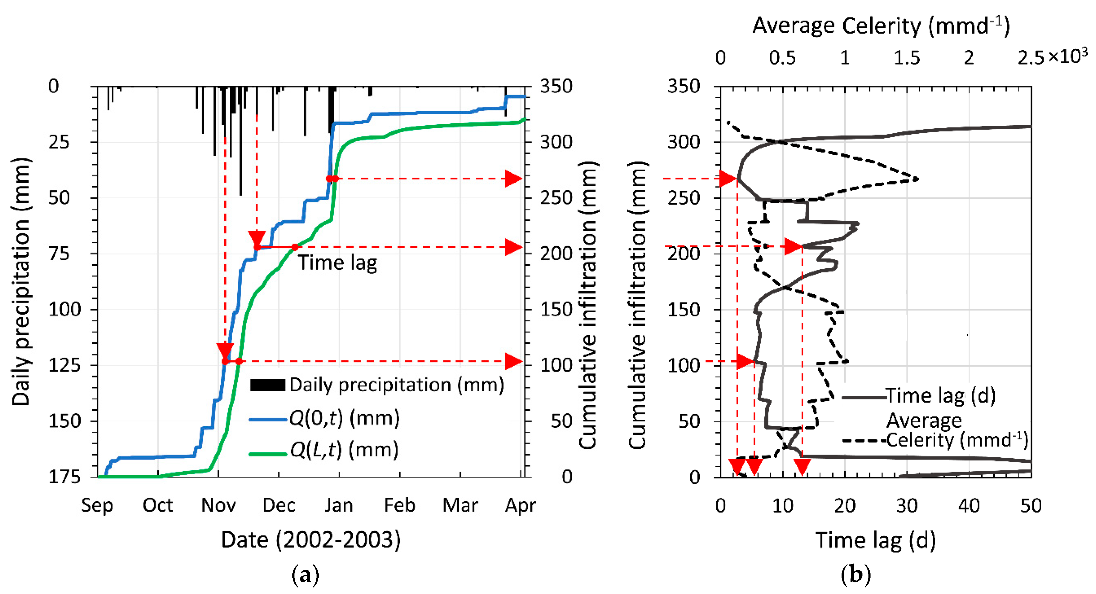
In order to investigate the effects of the characteristics of the episodic rainfall events on the infiltration processes along the preferential pathways, a comparative analysis between the daily precipitation, the infiltration rates at the topsoil q(0, t) determined according to the Equation (5) and the infiltration rate that reaches the water table q(L, t) according to the Equation (25) has been carried out. First, starting from q(0, t) and q(L, t) the cumulative curves of the infiltration at the topsoil Q(0, t) (L) and the cumulative curves of the infiltration at the water table Q(L, t) (L) have been built. They indicate the amount of the infiltrated water that crossed a certain surface (topsoil or water table) at a specific time. In other words, they indicate the time required to reach a determined amount of the infiltrated water.

Given a generic value of the cumulative infiltration, the time lag between Q(L, t) and Q(0, t) can be determined. It represents the travel time of the infiltrated water needed to reach the water table from the topsoil. Then, the average velocity of the wetting front (average celerity) can be determined as the ratio between the depth of the water table from the topsoil L and the determined time lag.

Figure 10a shows the cumulative infiltration at the topsoil and the water table for the time period 2002–2003. Moreover, the daily precipitation is reported. As shown in Figure 10a, for a generic value of the daily precipitation, the time lag between Q(L, t) and Q(0, t) can be measured. Then, at each time lag corresponds to a value of the cumulative infiltration.

The relationship between the time lag and the cumulative infiltration is shown in Figure 10b. Furthermore, the average celerity as function of the cumulative infiltration is reported.

In this way, each episodic rainfall event is related to the time lag and the average celerity, which represent the key parameters of the infiltration processes and the groundwater supply mechanism.

In correspondence to a significative rainfall event, the average celerity increases rapidly according to rainfall intensity. When a rainfall event passes, the average celerity decreases in a potential way, reaching a minimum value of 0.25 md⁻¹. The maximum values reached by the average celerity are strictly dependent on rainfall intensity. For all periods, average celerity is more or less equal to 500 mmd⁻¹ for lower intensity rainfall events and equal to 1800 md⁻¹ for higher intensity rainfall events.

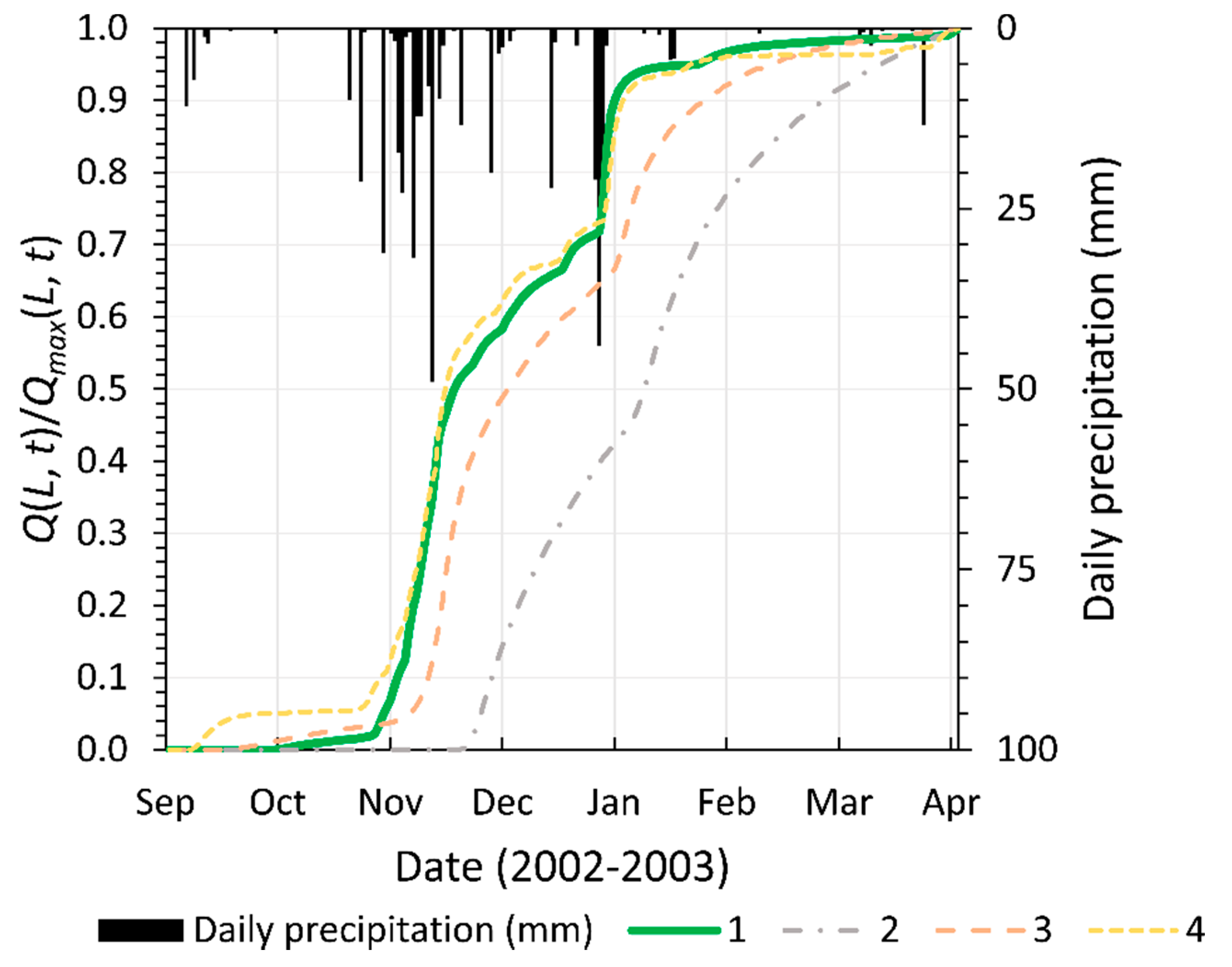
The results of the proposed infiltration model have been compared with the outputs of numerical simulations using the Brooks and Corey based Richards’ equation for a one-dimensional domain [41]. Infiltration occurs though the silty clay layer (5 m thick). Constant saturated hydraulic conductivity K_s (LT⁻¹), saturated volumetric water content θ_s (L³L⁻³), residual water content θ_r (L³L⁻³) and Brooks and Corey parameters such as the air entry pressure head h_d (L⁻¹) and the coefficient n (-) represent the hydraulic soil parameters of the implemented numerical model [42]. Steady state initial pressure head has been assumed to represent the most favorable condition for the infiltration dynamics. Groundwater level has been considered a constant overlapping the bed of the silty clay unit (5 m AMSL). The flux boundary condition has been applied at the topsoil equal to the hourly precipitation hydrograph. The silty clay unit has been assumed homogeneous and isotropic. Different configurations of the hydraulic parameters have been set. Figure 11 shows the relative cumulative infiltration at the water table obtained though the (1) kinematic dispersion wave model and the Brooks and Corey-based Richards’ model with the hydraulic parameters corresponding to (2) silty clay soil, (3) silty soil and (4) sandy soil.

The model results coming from the single domain homogeneous and isotropic one-dimensional Richards’ equation model were inconsistent with the observed hydraulic response, showing a time lag higher than the kinematic dispersion wave model did. Richards’ model closes in on the kinematic dispersion model only for the sandy soil configuration with a high value of the saturated hydraulic conductivity of 1.157 × 10⁻³ ms⁻¹—incoherent with the detected units. This supports the fact that the observed quick response of the aquifer was due to preferential flow mechanisms occurring in the vadose zone. A more complex heterogeneous and multi-porosity model based on Richards’ equation can improve the simulated response depicting the preferential flow paths mechanisms. However, the additional complexity required significantly greater data collection to estimate the model parameters.

5. Discussion

The present study has implemented an improved modeling framework for the analysis of the complex groundwater-level dynamics of an aquifer characterized by several singularities in its supply mechanism. The analysis of time series at the monthly scale (precipitation and groundwater level) followed the expected patterns, in which the terraced deposits fed the surficial aquifer through a long-term lateral recharge mechanism. Nevertheless, the analysis at the daily scale or less showed a behavior not explainable by this recharge mechanism alone. Long term lateral recharge combines with direct recharge through the vadose zone, giving rise to a quick response of the groundwater level.

The study area is susceptible to preferential flow due to different physical mechanisms involving the infiltration processes in the vadose zone at different spatial and temporal scales. The kinematic dispersion model captures the impact of the preferential flow mechanism at the field scale of the site. The model’s response is governed by three parameters. According to kinematic theory, the preferential diffusion index a should vary between 2 and 3. According to these two limits the conductance term b varies in the range between 3.6 × 10³ and 3.6 × 10⁴ mmh⁻¹.

The parameters a and b govern the celerity representing the velocity of the wetting front. As a decreases, b should increase in order to maintain the same order of magnitude of the celerity. A value of water dispersivity α_w equal to 200 mm was found. This parameter attenuates the infiltration wave, leading both to an infiltration rate hydrograph at the water table and the rising limb of groundwater level being more distributed in time.

The values found for the conductance term and water dispersivity are consistent with those found by [25,43] at laboratory scale. In the present study the maximum infiltration rate was equal to 6 mmh⁻¹—lower than those used by the authors presenting a minimum value of 30.35 mmh⁻¹. As a result, the conductance term is lower in this study according to the expected theoretic value. Anyway, the water dispersivity is higher. This is due to several factors linked to the scale dependence of dispersion phenomena. In an analogous manner to solute dispersion theory, water dispersion results are scale dependent. As the depth of the vadose zone increases, the probability that the wetting front moving downwards breaks up into more and more fingers increases. On the other hand, the capillary contribution to the wetting front movement can further attenuate the infiltration rate propagation. Moreover, as the depth increases, the conductance of the preferential flow pathways can be reduced. As a result, the infiltration rate hydrograph at water table is more attenuated.

The parameter q_crit indicates how much rain, occurring at high intensity, becomes recharged. The critical rate is 6 mmh⁻¹—mainly, the significant rainfall events occurred between 2003–2004 and 2004–2005. According to the source responsive theory [40], q_crit is equal to the product between a constant parameter that assumes a value of 2.1 × 10⁻⁶ m²h⁻¹ at temperature of water equal to 20 °C, and the smallest value of the facial area density M_min (L⁻¹) which characterizes the preferential flow path. Then in the present study a value of M_min equal to 2857 m⁻¹ was found. It represents the minimum fraction of the total specific surface area of the vadose zone on which preferential flow takes place. This parameter measures the susceptibility of a field site to preferential flow. Cuthbert et al. 2013 found a value of M_min between 250 and 750 m⁻¹ at field site in Shropshire (UK) [44]. Nimmo 2010 found a value of M_min equal to 4000 m⁻¹ for Masser site in Pennsylvania [40].

Local surface depressions due to the presence of several reclamation channels in the study area play an important role in the preferential flow mechanism at the areal scale [38]. During rainfall events, water accumulates in the reclamation channels, increasing the opportunity for preferential flow.

The velocity of the wetting front (average celerity) is strictly correlated with the rainfall intensity. Its maximum value is in the range between 1500 and 2000 mmd⁻¹, which is consistent with the value reported for preferential flow in [38]. The comparison between the observed groundwater levels and simulated ones highlighted a delay in the rising period of the simulated groundwater level with respect to the observed one that systematically occurred at the first rainfall event of each investigated time series. This can be ascribed to the fact that the value of mobile water content is assumed equal to zero at the beginning of simulation, underestimating the speed of the infiltration wave. Anyway, since the time series begin just after the dry season, the imposed initial condition should not be very different from the real case. Another explanation can be attributed to the fact that the velocity of the wetting front is greater when the soil is dry, in contrast with the theory that higher antecedent soil moisture condition hydraulically activates the preferential pathways [45,46]. However, several authors support the theory that when the soil is dry, preferential flow is more evident [47]. With less antecedent soil moisture, shrinkage cracks play an important role in rapid and deep water movement through dry soil. Water backfills the shrinkage cracks, increasing the opportunity for preferential flow via preferential pathways caused by wetting instability due to the compression of air below the accumulated water into the shrinkage cracks. With more antecedent soil moisture, preferential flow is more dominated by the stable preferential pathways. Lateral flow from macropores to the soil matrix reduces, and as a consequence the amount of preferential flow and number of channels increase.

When the groundwater level affects less permeable strata, a lower value of the storage coefficient is found due to the presence of aquitards represented by the surficial silty and clay unit that locally confine the shallow aquifer. Changes in storage coefficient affect the amplitude of the groundwater level fluctuation. The conducted analysis discloses the presence of a transition zone at depth from topsoil equal to ≈5 m BGL that corresponds to the bottom of the surficial silty clay unit detected at the site. Storage coefficient decreases passing from 0.3 to 0.08 evidence a transitional behavior where confined and unconfined conditions coexist. Then the surficial aquifer passes from unconfined condition to weakly confined condition and vice versa.

6. Summary and Conclusions

The present study presents the complex groundwater-level dynamics of the surficial level of the Ionian coastal aquifer in southern Italy. We analyzed the articulate groundwater supply mechanism. An improved modeling framework based on kinematic dispersion wave theory has been used to simulate water flow through preferential paths and predict groundwater level fluctuations in a surficial aquifer, which occasionally can flow in a weakly confined condition. The prediction accuracy evaluation and comparison indicated that the kinematic dispersion wave model and its numerical solution with the proposed particle-based model are able to capture the preferential flow recharge mechanism in the study area, showing good agreement with the observed groundwater level time series.

The local stratigraphic sequence is characterized by a surficial thin silty and clay level covering the loamy sandy levels hosting the aquifer. Therefore, the direct recharge could appear quite difficult for the presence of a low permeability level covering the high permeability levels hosting groundwater. The recharge could be attributed partly to the coarse-grained deposits associated with the terraced deposit outcroppings about 1200 m upstream that are hydraulically connected with the coastal aquifer system. Anyway, the response of groundwater level is almost immediate, so that it cannot be due only to lateral recharge, but also some mechanism of direct supply. Thus, the study area is subject to infiltration through preferential flow paths due to different physical processes at spatial and temporal scales. At the areal scale, the presence of several reclamation channels widespread in the plain cuts the thin layer of low permeability deposits, leading to local topographic depressions that encourage the opportunity of the preferential flow.

Moreover, the conversion from unconfined to weakly confined groundwater flow was highlighted. When the groundwater level rises above the bottom of the silty and clay unit, weakly confined condition occurs. The storage coefficient reduces from 0.3 to 0.08. These estimated values are coherent with a critical rainfall rate q_crit of 6 mmh⁻¹.

Recharge via preferential flow path is strictly correlated with the precipitation characteristics in terms of duration, magnitude and intensity. In the study area, intense rainfall events favor direct recharge of the surficial aquifer via preferential flow dynamics, but at the same time reduce the travel time of the mobile water in vadose zone, increasing the risk of surficial groundwater contamination as a consequence of preferential flow.

The comparison between model prediction and observed data indicates that the susceptibility of preferential flow in the study area results is relatively high. The results evidence the influence of moisture antecedent conditions on preferential flow mechanisms. Antecedent dry conditions seem to favor preferential flow via shrinking cracks.

It is evident that a complex set of hydraulic processes control the surficial aquifer supply. Both lateral/upward recharge and direct recharge via capillary-dominated matrix flow and preferential flow processes interact with each other to give the observed hydraulic response. The state-of-the-art of the Richards’ equation models require many input flow parameters to describe the heterogeneity of the media. This type of model and the relative computational demands may be of the little practical use for estimating groundwater recharge at the field scale. The developed modeling framework represents a practical modeling approach for estimating the direct recharge due to the episodic rainfall events.

Future development of this study will regard the implementation of precise weighting lysimeters in the study area to observe and analyze the preferential flow processes at several depths in the vadose zone. Furthermore, transient test analysis is recommended in order to deepen the understanding of the mixed unconfined–weakly confined groundwater behavior.