Carbon Balance and Streamflow at a Small Catchment Scale 10 Years after the Severe Natural Disturbance in the Tatra Mts, Slovakia

Abstract

Natural disturbances (windthrow, bark beetle, and fire) have reduced forest cover in the Tatra National Park (Slovakia) by 50% since the year 2004. We analyzed carbon fluxes and streamflow ten years after the forest destruction in three small catchments which differ in size, land cover, disturbance type and post-disturbance management. Point-wise CO₂ fluxes were estimated by chamber methods for vegetation-dominated land-use types and extrapolated over the catchments using the site-specific regressions with environmental variables. Streamflow characteristics in the pre- and post-disturbance periods (water years of 1965–2004 and 2005–2014, respectively) were compared to identify changes in hydrological cycle initiated by the disturbances. Mature Norway spruce forest which was carbon neutral, turned to carbon source (330 ± 98 gC m⁻² y⁻¹) just one year after the wind disturbance. After ten years most of the windthrow sites acted as carbon sinks (from −341 ± 92.1 up to −463 ± 178 gC m⁻² y⁻¹). In contrast, forest stands strongly infested by bark beetles regenerated much slowly and on average emitted 495 ± 176 gC m⁻² year⁻¹. Ten years after the forest destruction, annual carbon balance in studied catchments was almost neutral in the least disturbed catchment. Carbon uptake notably exceeded its release in the most severely disturbed catchment (by windthrow and fire), where net ecosystem exchange (NEE) was −206 ± 115 gC m⁻². The amount of sequestered carbon in studied catchments was driven by the extent of fast-growing successional vegetation cover (represented by the leaf area index LAI) rather than by the disturbance or vegetation types. Different post-disturbance management has not influenced the carbon balance yet. Streamflow characteristics did not indicate significant changes in the hydrological cycle. However, greater cumulative decadal runoff, different median monthly flows and low flows and the greater number of flow reversals in the in the first years after the windthrow in two severely affected catchments could be partially related to the influence of the disturbances.

1. Introduction

In addition to wood supply, forest ecosystems provide a multitude of benefits in terms of climate and water regulations, carbon sequestration, freshwater quality, soil protection, nutrient cycling, human health, recreation, biodiversity, wildlife habitats and many other. The ability of forest ecosystems to provide these ecosystem services (ES) is very much dependent on their status, structure and functioning [1]. In the last decades, forests have been globally affected by more frequent disturbances [2] due to which many ES are supposed to be threatened [3]. This trend is believed to continue in the future because of the ongoing climate changes [4,5,6]. Changes in the climate system will change an overall redistribution of precipitation [7] and alter the partitioning of carbon uptake and loss [8].

The role of forests in carbon sequestration has been acknowledged in many studies [9], forest and landscape projects [10]. Forest disturbances change carbon fluxes resulting from the difference between carbon uptake by vegetation (gross primary photosynthesis, GPP) and loss by ecosystem respiration (RE). This difference, the net ecosystem exchange (NEE), indicates whether the ecosystem is sequestering or emitting carbon to the atmosphere. Initially, most disturbances shift ecosystems to being a carbon source, while recovery is usually associated with greater carbon storage [11,12,13,14,15]. The duration and dynamics of these fluxes depend on the kind of disturbance and its intensity [16,17]. Recently, climate change-induced changes in carbon sequestration have been intensively studied (e.g., [18,19,20,21]), and the results show the role of site-specific conditions and the influence of silvicultural methods [22,23]. Less attention has been given to post-disturbance forest management impact on carbon fluxes, although the role of reforestation in carbon sequestration is widely recognized [9].

The most commonly used method for ecosystem or landscape-scale estimation of carbon balance is the eddy-covariance (EC) technique [24,25]. Despite recent technical and methodological advances [26] this method has still some limitations, especially in complex terrains. An alternative approach, particularly suitable in heterogeneous landscapes, is the chamber method which is low-cost and easy to apply. Chamber measurements range from leaf to entire plant flux estimations. They were successfully used for validation of the EC technique [27]. However, small spatial coverage of the chamber method requires a large effort to collect sufficient data needed to develop simple empirical equations to scale up the results to the entire ecosystem [28]. At the same time, the chamber-based flux estimation is subject to uncertainties related to site (soil, microclimate) heterogeneity, that are further increased by heterogeneous disturbance patterns.

Plant assimilation and evapotranspiration are regulated by canopy stomatal conductance. Plant canopy in carbon-water coupling models is often abstracted as a big leaf. Such a simplification in some implications is in conflict with the clumped canopy structure. A two-big-leaf scheme and two-leaf scheme that stratify a canopy to sun-exposed and shaded leaves have been developed to make the big leaf concept more applicable [29].

Forest disturbances do not affect only carbon fluxes. They have a direct effect on the main components of catchment water balance, i.e., precipitation (interception) and evapotranspiration (e.g., [30]). Consequently, runoff generation, snow accumulation and melt, groundwater recharge or catchment runoff characteristics can be altered, e.g., [31,32,33]. Catchment runoff is an integrated result of hydrological processes taking place in a catchment. Runoff data series are therefore often analyzed to identify the effects of forest disturbances on catchment hydrology by comparing flow characteristics before and after the disturbance. A number of studies analyzing the influence of deforestation concluded that peakflow or low flow characteristics temporarily increased after deforestation, e.g., [34,35,36] and that deforestation had to affect a larger area (e.g., at least 20% of the catchment) to show the effects in runoff records [34,37]. These conclusions were often obtained by comparing flow characteristics in paired catchments, in which one catchment was subjected to forest harvesting. Alila et al. [38] contend that in paired catchments the effects of forest harvesting on floods should be evaluated considering simultaneous changes in both magnitude and frequency of the floods. In their study, floods are understood as a subset of peakflow frequency distribution containing flows with the magnitude exceeding channel capacity and return interval of 1–10 years or more.

In addition to peakflow, low flow or water yields traditionally used in the forest harvesting impact studies, many indicators were developed in environmental flow studies to characterize impacts of river regulations. The commonly used IHA tool (Indicators of Hydrologic Alteration) [39] calculates 67 characteristics based on data series of daily discharge. They characterize magnitude and duration of monthly, annual and extreme water conditions. Olden and Poff [40] examined 171 indices describing magnitude, frequency, duration and timing and rate of change in flow events (including those from IHA) using long-term flow records from 420 sites across the continental USA. They found out that the majority of indices were highly inter-correlated and proposed sets of selected indices that adequately characterize flow regimes in a non-redundant manner for different stream types. Gao et al. [41] concluded that metrics termed ecodeficit and ecosurplus [42] based on a flow duration curve can provide a good overall representation of the degree of alteration of streamflow time series.

Even though carbon and water balance are coupled processes, they are rarely compiled at a catchment scale [8]. Such an analysis is missing also in the Tatra Mountains literature where intensive research of multiple disturbing factors impact on the forests has resulted in numerous studies and publications. Our work attempts to fill the gap in existing studies by evaluating spatially integrated information on ecosystem dynamics at a landscape scale.

The main aim of this study is to evaluate carbon balance and to examine streamflow characteristics in three small catchments in the Slovak part of the Tatra Mountains ten years after the extraordinary wind disturbance that initiated vast forest destruction in the area. Secondary objectives of this study are: (i) to estimate CO₂ fluxes with chamber and biometric methods in different ecosystem (landscape) types and under different post-disturbance management, (ii) to extrapolate C balance from point-wise to the catchment scale, and iii) to evaluate changes in catchment runoff. We hypothesized that (a) intact forest acts as a carbon sink, (b) forest disturbances stimulate immediate large carbon losses from forests and subsequent gradual recovery of carbon balance, and (c) disturbances change certain flow characteristics.

2. Material and Methods

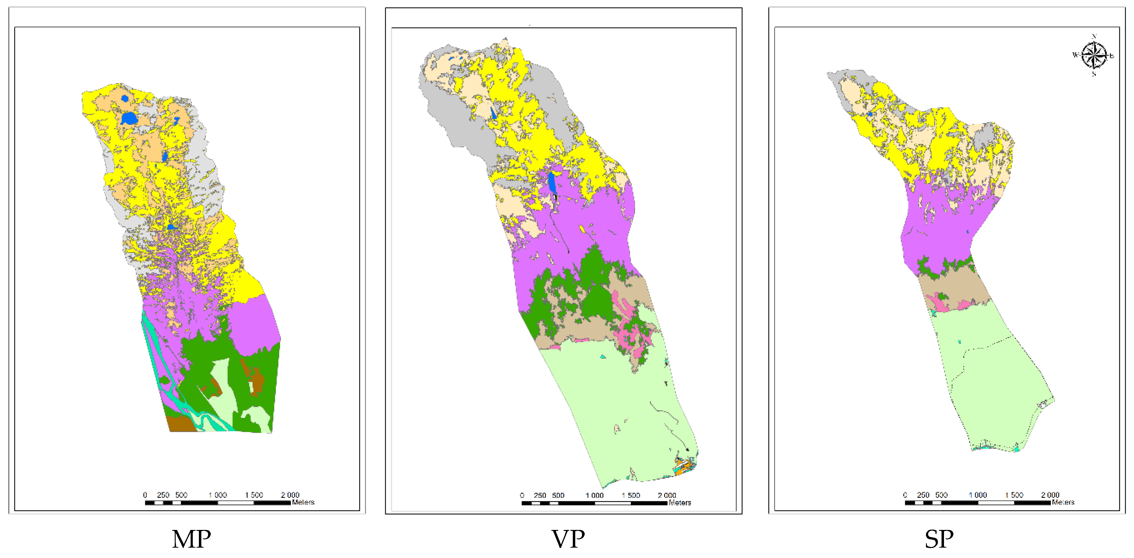
2.1. Study Sites

Tatra Mountains is the highest mountain range of the Carpathians and a regional water tower of northern Slovakia and southern Poland. The majority of the territory is protected within the Tatra National Park, Slovakia (TANAP) and Tatrzański Park Narodowy, Poland. The TANAP protects also natural and seminatural predominantly Norway spruce forest that covers approximately 40,000 ha. Roughly 30% of the forests is strictly protected in the no management zone. A downslope wind locally named “bora” sporadically hits forest stands on the lee side of the mountains [43] and causes large destructions. In November 2004, more than 12,000 ha of mature forests was destroyed by such an extremely strong windstorm. Smaller windstorms and bark beetle outbreaks initiated by the 2004 windthrow damaged additional 7000 ha of the forests in the following years. In total, 50% of mature forest stands were damaged during the 2004–2014 period in the Tatra National Park (www.lesytanap.sk, accessed on 1 July 2020).

Three small catchments with long streamflow records were selected for this study (Figure S1). The catchments are located on the southern (lee) slopes of the Tatra mountains and differ in their areas and proportion of ecosystem types (Figure 1). The 2004 windfall significantly reduced forest cover in two catchments (the Velický and Slavkovský Creek catchments, hereafter denoted as VP and SP), while forests in the third catchment remained almost unaffected by the windfall (the Mlynický Creek catchment, hereafter MP). The catchments are built by crystalline rocks that are partially covered by Quaternary sediments and by glaciofluvial sediments (moraines) at higher and lower elevations, respectively. Soils are generally stony, well drained, mostly shallow, very acid and poor in nutrients [44,45]. Lithic Leptosols and Hypersceletic Regosol are dominant above tree line. Haplic Podzols and Dystric Cambisols (WRB classification) are dominant forest soil types. Extremely rocky soils (rankers) cover ca 30% of the forest area [45].

Vegetation at the highest elevations (above 1700 m a.s.l.) is sparse and dominated by Agrostis pyreneica, Juncus trifidus, Avenella flexuosa, Avenula versicolor, Luzula sudetica. Mountain pine (Pinus mugo) forms a continuous belt above the tree line (1550 m a.s.l.) and grows up to 1700 m a.s.l. with Avenella flexuosa and Calamagrostis villosa under the canopy. The area between 900 and 1500 m a.s.l. was almost completely covered by mature forests (Lariceto-Piceetum and Sorbeto-Piceetum communities) before the disturbances. Norway spruce (Picea abies) was the dominant tree species (covering 70–90%), while European larch (Larix decidua) covered 10–30% of the forest in the studied catchments [44].

The long-term annual average temperature ranges from 5.3 °C (850 m a.s.l.) to 1.7 °C (1750 m a.s.l.) Annual precipitation total ranges from 800 mm up to 1350 mm with maximum in summer months [45]. Study catchments are shown in Supplement, Figure S1. For carbon study, only the upper parts (micro catchments) of the entire catchments were chosen, as presented in Figure 1.

The carbon study areas feature typical land cover types that are hereafter termed as types of ecosystems. They are represented by tarns and streams, alpine meadows, dwarf mountain pine stands, undisturbed mature Norway spruce forests, managed 10-year-old windthrow, unmanaged 10-year-old windthrow, managed 1-year-old windthrow, standing/lying trees killed by bark beetle, burnt windthrow and non-vegetation types (rocks, roads, buildings, etc.) Ecosystem types were classified by ArcGIS from the aerial orthophoto maps created in 2015. The areas of ecosystem types in the catchments used in the carbon balance evaluation are given in

Table 1. Total catchment area (km²), portion of deforestation in 2004 and carbon study areas (ha) with proportion (%) of ecosystem types in the mountain parts of study catchments in 2015; MP—the Mlynický Creek catchment, VP—the Velický Creek catchment, SP—the Slavkovský Creek catchment; ROC—rock slopes, DEB—debris and moraines, WAT—water, ALM—alpine meadows; DWP—dwarf pine; IPS—area affected by the bark beetle outbreaks; REF—mature forest unaffected by the 2004 windthrow; EXT—extracted windthrown area; FIR—windthrown area affected by subsequent fire; NEX—non-extracted windthrown area; REX—extracted 1-year-old windthrow.

Catchment	Total Area [km2]	Total Forest Reduction [%]	C Study Area [ha]	ROC	DEB	WAT	ALM	DWP	IPS	REF	EXT	FIR	NEX	REX
Color in Figure 1
MP	83.0	5.0	758.7	11.6	16.6	0.8	25.7	21.2	2.1	14.6	4.6	0.0	0.0	0.01
VP	58.0	20.0	1031.7	13.3	10.0	0.3	14.1	16.8	7.3	8.1	27.5	0.0	1.7	0.01
SP	43.0	32.0	612.1	5.6	15.1	0.1	16.0	18.7	6.3	1.4	7.9	27.7	0.9	0.01

.

Vegetation (ALM, DWP, mature intact REF forest, and disturbed IPS, EXT and NEX ecosystem types) together covered 72% of the catchment area in MP, 76% in VP and 79% in SP. Pre-disturbance forest cover was 160.7 ha in MP, 461.1 in VP and 270.2 ha in SP. Until 2014 forest cover decreased from 21% to 14% in MP, from 45% to 8% in VP and from 44% to 1% in SP. Thus, the most heavily affected forest stands were in the SP catchment, where total forest cover was reduced by 98%.

Most of the forests affected by disturbances were managed. Post-disturbance forestry operations focused on slash harvest and reforestation. Only small patches remained unmanaged, namely 1 ha in MP, 9 ha in VP and 7.2 ha in SP catchment. These numbers include also forests killed by consequent bark beetle attack in the no management zone of TANAP. In 2014, strong winds damaged forest edges of the 2004 windthrow. This event offered an opportunity to study carbon dynamics immediately after the disturbance. We use the abbreviation REX to refer to this type of ecosystem, which is not shown in Figure 1 due to the limited size of patches and spatially distributed occurrence of this ecosystem type.

The conditions in our study differ from studies devoted to impacts of forest harvesting on streamflow. In our case the primary forest disturbance was natural and instantaneous (it occurred within a few hours on 19 November 2004), and was followed by subsequent disturbances (bark beetle outbreak, local fires and other smaller windthrows). The urbanization of the disturbed area is low, and there is no flow regulation. As it is quantified above, the windthrow damaged a large forested area. Due to the timing of the disturbance and the beginning of winter, most of the wood windthrown wood remained on the ground until spring 2005. Thus, the highest potential flood hazard related to forest removal was approximately in the period between autumn 2005 and winter 2006. The flood hazard declined in the following years due to vegetation regrowth (both natural and managed). Holko et al. [46] compared water balance, minimum and maximum runoff, runoff thresholds, number of runoff events and their selected characteristics, runoff coefficients, and flashiness indices before (starting with the water year 1962) and after the windfall (until the water year 2007) in eight catchments of the disturbed area. The impact of deforestation was not clearly manifested in the analyzed hydrological data. Analysis of baseflow variability [47], runoff response to heavy rainfall [45] and flow duration curves [48] resulted in the same conclusions although [48] concluded that discharges with the highest probability of exceedance (Q90% and Q80%) in the decade following the windfall (2005–2014) occurred more frequently than in period 1965–2004. Most of the above analyses were based on a shorter time series of data after the first disturbance (windthrow). In this article we used additional indices that were not used in the previous studies. Longer data series also allowed additional analysis of the occurrence of peakflows with different return periods.

Evaluation of carbon balance was based on manual CO₂ fluxes measurement by chamber methods during the growing season 1 April–31 August 2014. Meteorological and phenological data were recorded all year round. Changes in catchment streamflow were evaluated using daily discharge data from water years 1965–2014 measured in the national network operated by the Slovak Hydrometeorological Institute.

2.2. Meteorological and Hydrological Data

Climatic data are commonly used as a proxy for estimation of carbon fluxes. Hourly measurements of air temperature and humidity at a standard height of 2 m above the terrain (Hygroclip, Switzerland), soil temperature at 2 cm and 10 cm depths (107 Campbell, UK), soil moisture at 10 cm (theta Ml2x, Delta UK), photo synthetically active radiation (PAR Quantum Skye, Ireland) and precipitation (Davis, CA, USA) were recorded by the Campbell data loggers (Campbell, UK). Mobile meteorological stations were located at 1150 m a.s.l. in all studied catchments. Additionally, instant soil temperatures (at 2 cm and 10 cm depths), soil moisture (0–6 cm) and PAR were recorded concurrently with CO₂ flux measurements. Daily discharges measured at catchment outlets in period 1965–2014 were provided by the Slovak Hydrometeorological Institute.

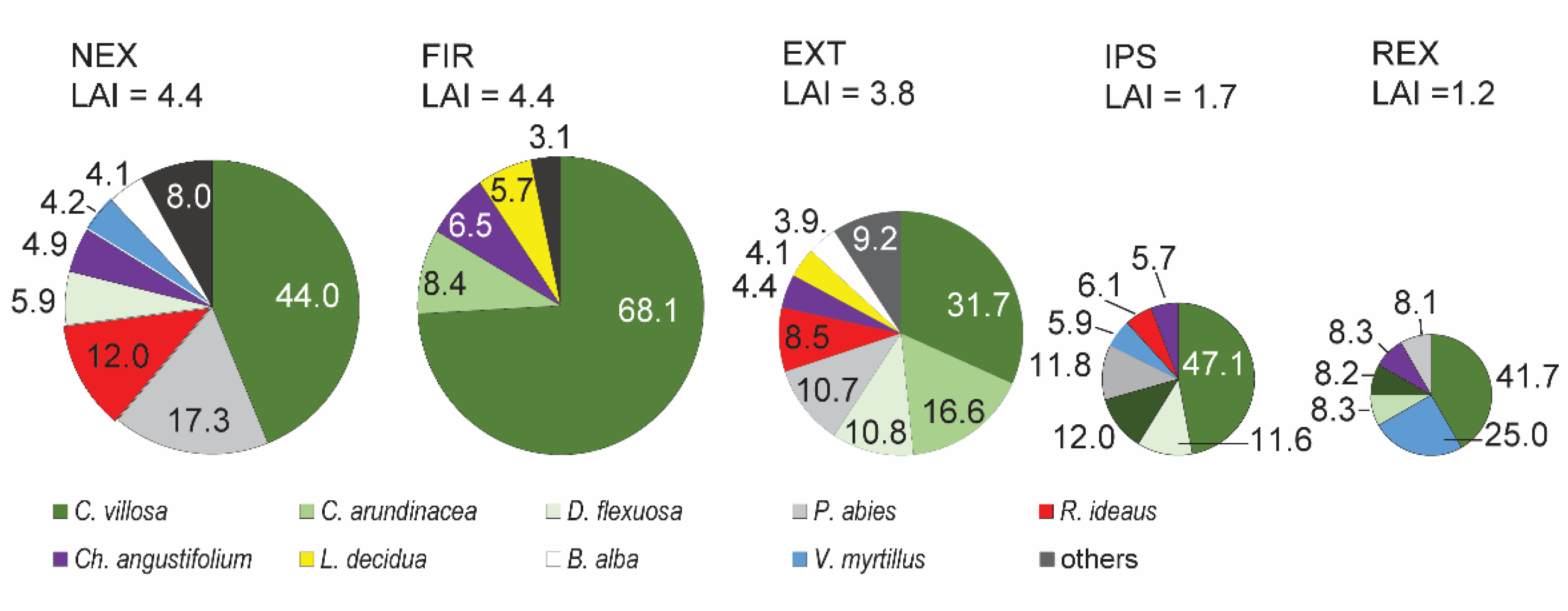
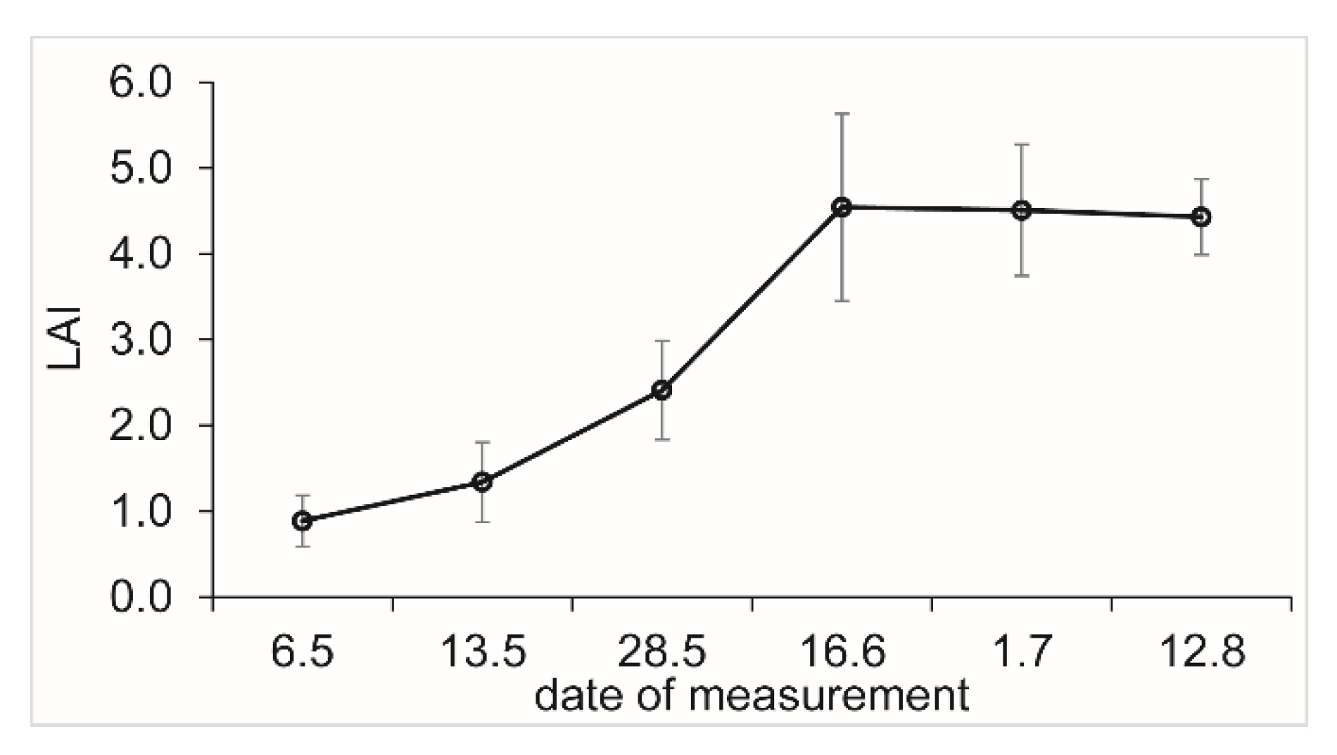
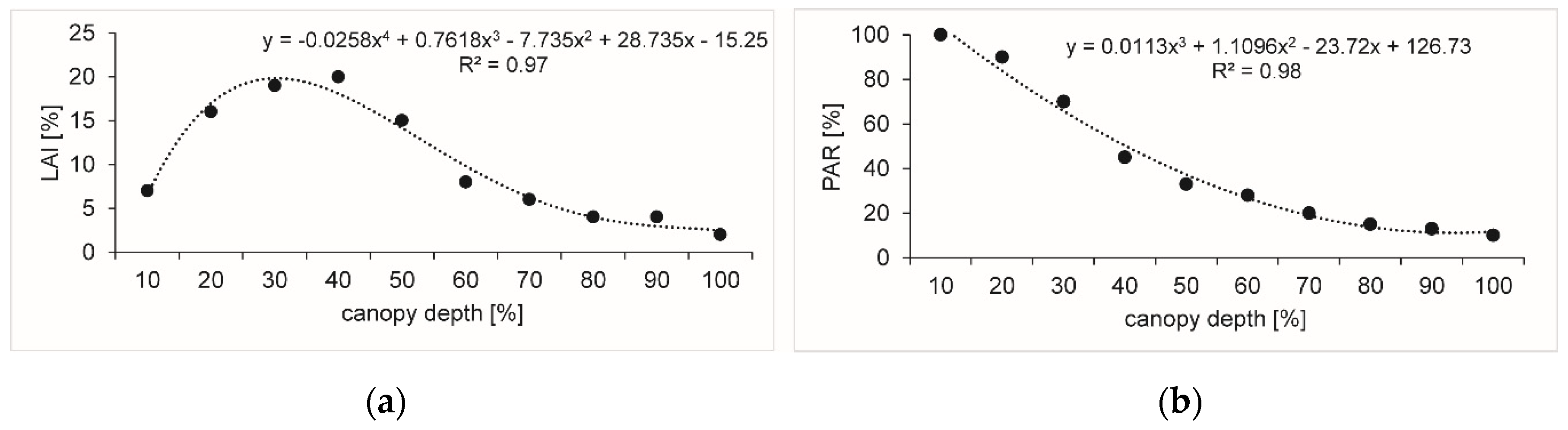
2.3. Vegetation and Phenology

Qualitative (species composition) and quantitative (biomass, coverage) vegetation parameters are the most important predictors of plant assimilation. Species composition in relevant ecosystem types was derived as a species-specific contribution to total leaf area index (LAI). Species-specific and total LAI were used for a big leaf model construction. In this study the big leaf model is three-dimensional with distinct vertical distribution of LAI and available PAR.

Plots for vegetation sampling were established along 21 transects, each 540 m long, located in the DWP, IPS, REF, EXT, FIR, NEX and REX ecosystem types. The plots were set up every ten meters and each plot consisted of three squares of different size: 0.04 m² for grass and herbs, 0.25 m² for shrubs and 25 m² for trees. During the peak of the growing season (mid-June–end of July), grasses, herbs and shrubs were clipped, scanned, dried at 60 °C for 48 h and weighted in the laboratory. First, we estimated species-specific leaf area (SLA) from a regression between the foliage biomass and the foliage area. Plant leaf area of scanned leaves (40–50 samples for each species, each sample contained 10–50 leaves) was calculated by the ImageJ software [49]. Species-specific leaf area index (LAI) was derived by multiplying foliage biomass and SLA. Sum of species-specific LAI gave total site LAI. Tree diameters near the ground surface and height of each tree were measured with digital clipper and telescopic sticks, respectively. Tree foliage biomass was derived from biomass regressions proposed by [50,51,52,53]. Vertical distribution of LAI on dominant plant species was measured with Licor 2200 Plant Canopy Analyser in 10 cm vertical categories from the top of the canopy to the ground. Licor 2200 was also used for the estimation of temporal changes along established vegetation transects (on 5 × 5 m squares) and verification of total LAI.

The dates of bud break, first and full leaves development were recorded and kindly provided by the phenology observation stations of the Slovak Hydro Meteorological Institute located in the MP catchment.

2.4. Carbon Balance

Carbon balance (net ecosystem exchange, NEE) refers to the amount of carbon captured by plants. We estimated NEE as a difference between assimilation (GPP) and ecosystem respiration (RE). Assimilation was estimated during growing season (1 April–31 August). Respiration was measured all year round, except for the snow cover period (mid December–early March). Negative sign in NEE represented carbon uptake, while positive sign for carbon efflux. Spatial extrapolations of leaf, plant and point-wise carbon flux data to the catchment scale were based on regressions with actual vegetation. Temporal extrapolation of instant carbon fluxes was based on their regression with meteorological data and plant phenological development [54].

2.4.1. Assimilation—GPP

GPP was estimated as a sum of net exchange (NEE) and respiration (RE) directly measured by the chambers. We used leaf or whole plant gas measurement for dominant plant species accordingly to the plant size and shape. GPP refers to the amount of CO₂ captured by leaves (µmol C m⁻² s⁻¹) which is usually mainly controlled by available PAR [µmol photons m⁻² s⁻¹]. This response is expressed by the light response curves which were constructed for dominant plant species. The light response curve defines light saturated assimilation (GPP_max) and quantum yield (α) which naturally change during season. For this purpose, we repeated field measurements of GPP_max and α of most plant species on a 2-week basis, and once a month for conifer trees. GPP_max was derived from plotted light curves and α was calculated using the nonlinear regression (Statistica 12). The Michelis – Menten type of regression [54] was used for calculation:

$$GPP=\frac{GP{P}_{max}\times \alpha \times PAR}{GP{P}_{max}+\alpha \times PAR}\times LAI$$

(1)

GPP was calculated on an hourly basis. As incoming PAR changes continuously, we used 60 min averages to calculate hourly and consequently daily and total (seasonal) GPP. As the shaded leaves inside the canopy receives only portion of incoming PAR, we divided the canopy into 10 cm vertical sections and measured incoming PAR from the canopy top to the ground (100 measurements per species) by Quantum sensor. Similarly, LAI vertical distribution across the canopy was measured by Licor 2200. Empirical models of vertical LAI distribution and PAR dissipation for dominant species were applied to correct GPP derived from leaf measurements.

Leaf measurements: Licor 6400XT device was used for the gas exchange measurement on wide leaf plants. The samples (20 leaves per species, equally at both sunny and shaded sides) were exposed to different intensities of PAR (0, 50, 100, 200, 400, 800, 1200, 2000 µmol photons m⁻² s⁻¹) to construct the light response curves. The leaf CO₂ net exchange was measured biweekly on dominant species; the parameters are shown in Table S1.

Plant measurements: Customs built plexiglass chambers of 16 and 60 dm³ were used to measure the whole plant gas exchange on narrow leaf plants (grasses). The chambers were equipped with GMP 343 CO₂ sensor (Vaisala, Finland), PAR, temperature and air humidity probes and a small fan. Incoming radiation was modified with a variable combination of shading nets. Each measurement lasted two minutes. Only the linear part of the CO₂ concentration change was used for the calculation of CO₂ flux following the ideal gas law [55].

Mature forest estimation: The GPP in mature spruce forest was calculated with annual wood stock increment (m³ ha⁻¹). Average annual wood stock increment was derived from permanent research plots located in studied catchments [56]. Allometric and biomass expansion factors were used to transform wood stock increment to net primary productivity (NPP) according to [7] and [57]:

$$NPP=V\times D\times BEF\times k\times c$$

(2)

where V—annual wood stock increment, D—wood density, BEF—expansion factor for above-ground biomass, k—coefficient for below-ground biomass, and c—portion of C in wood.

The GPP is equal to NPP divided by carbon use efficiency coefficient (CUE), GPP = NPP/CUE. We used the CUE value for Norway spruce according to [58].

2.4.2. Ecosystem Respiration—RE

Ecosystem respiration (RE) is the sum of soil and aboveground plant respiration. Soil respiration (SR) was measured on fixed collars with a PVC custom-built dark closed chamber (diameter 30 cm, height 10 cm) equipped with Vaisala GMP 343 CO₂ probe and a small fan. The CO₂ concentration was measured every five seconds for five minutes and corrected for air pressure, temperature and humidity. Soil temperature and soil moisture were recorded along with the SR measurement. SR was measured every two weeks along fixed transects (for details see [54]). For this study we used the location and the number of sampling points (collars) as shown in

Table 2. Numbers of sampling points for estimation of soil respiration in different ecosystems.

Ecosystem Type	Abbreviation	Number of Points	Altitude (m a.s.l.)
Alpine meadow	ALM	3	1730
Dwarf pine	DWP	5	1550
Bark beetle attacked forest	IPS	10	1180
Mature undisturbed forest	REF	20	1200
Windthrow extracted	EXT	24	1100
Burnt windthrow	FIR	8	1100
Windthrow non-extracted	NEX	8	1100
1-year-old windthrow	REX	8	1100

.

Measured SR values were fitted with an exponential function based on soil temperature [59]:

SR = k × e^{a X T}

(3)

SR was calculated for each individual sampling point (collar), where T is soil temperature in 10 cm, k and a are regression parameters of the function derived by nonlinear regression using Statistica 12. Only statistically significant parameters (p < 0.05) were employed for SR modelling. The annual SR model was based on extrapolation of instant SR values using continuously measured soil temperature in 10 cm depth. Each ecosystem type was represented by an average calculated from all measured points.

Leaf respiration was measured with Licor6400 XT as species-specific leaf net CO₂ exchange under dark conditions (PAR set to 0). Stem (wood) respiration was measured on collars permanently fixed to the trunks (n = 5) on trees with average height and diameter. The measurements were realized on a 2-week basis. Arithmetic means of measured values were used to derive regressions with air temperature similarly as for soil respiration and to calculate component (leaves, stem) and annual ecosystem respiration.

2.4.3. Flux Data Validation

Confidence intervals for estimated CO₂ fluxes were calculated with the Monte Carlo method as proposed by Knohl [60]. First, we calculated the regressions in Equation (3) for all components of ER (soil, stem, leaf) and their standard deviations (SD). Second, we calculated 5000 seasonal sums of respiration based on measured temperatures and 5000 combinations of k and a parameters sampled by the replacement from bivariate normal distribution defined by the values and SD of k and a. A similar approach was applied to estimate GPP uncertainty. The GPP_max and α parameters in Equation (1) were estimated using nonlinear regression. The seasonal sum of GPP based on hourly PAR for different plant species was calculated with 5000 combinations of GPP_max and α parameters sampled using the same method as described above. The overall catchment scale confidence intervals for NEE were calculated as a square root of the weighted sums of partial ecosystem level CIs.

2.5. Streamflow Characteristics

Daily discharge data from the water years 1965–2014 were analyzed. The MP catchment represented a small mountain headwater catchment that was unaffected by the 2004 windthrow while the VP and SP represent catchments that were significantly affected by the windthrow and consecutive bark beetle outbreak and fire disturbances. Having data from ten water years after the windthrow, we first examined decadal cumulative runoff from 1965 to 2014 and compared it to cumulative precipitation from the only two precipitation stations existing in the study area that provide representative data from higher elevations (Skalnaté Pleso and Kasprowy wierch).

The IHA indicators were also examined visually (magnitudes, ranges, temporal trends and abrupt changes) with the aim to identify the influence of the disturbances on the low and high flow characteristics (annual minima: 1-day, 3-day, 7-day and 30-day annual minima, 1-day, 3-day and 7-day annual maxima), baseflow index, environmental flow components (frequency and duration of high and low flow pulses), rate and frequency of flow changes (rise, fall, number of reversals). High flows were defined as flows that exceeded 75% of all daily flows. Low flows were flows equal to or less than 50% of all daily flows. The number of reversals represents the number of flow changes from falling to rising and vice versa per year. Median values of all characteristics in the decades of 1965–2014 were compared as well.

Characteristics recommended by Olden and Poff [40] for perennial streams with snow and rain regime (

Table 3. Selected indicators of flow regime changes proposed for the evaluation of perennial streams with snow and rain regime by [40].

Code	Definition
MA3	coefficient of variation in daily flows
MA44	variability in annual flows divided by median annual flows; the variability is calculated as 90th minus the 10th percentile
ML13	coefficient of variation in minimum monthly flows
ML22	mean annual minimum flows divided by catchment area
MH17	mean of the 25th percentile from the flow duration curve divided be median daily flow across all years
MH20	mean annual maximum flow divided by catchment area
FL3	total number of low flow spells (threshold equal to 5% of men daily flow) divided by the record length in years
FL2	coefficient of variation in the low flow pulse count (below 25th percentile)
FH3	high flow pulse count (high flow pulse is 7 times the median daily flow)
FH5	mean of high flow events per year (high flow is 1 times the median flow)
DL6	coefficient of variation in annual minima (1-day annual minima)
DL13	mean annual 30 day minimum divided by median flow
DH12	mean annual 7-day maximum divided by median flow
TL1	mean Julian date of the 1-day annual minimum flow over all years
RA9	coefficient of variation in number of reversals
RA8	number of positive and negative changes in water conditions from one day to another (flow reversals)

) were then calculated and analyzed as well. Except for the number of flow reversals, those characteristics were not used in the study area in our earlier studies.

Our final group of streamflow analyses focused on the occurrence of flows with specified probability of exceedance estimated from the flow duration curves. A flow duration curve is a cumulative frequency curve that characterizes probability of exceedance of specified discharges during a given period [61]. First, decadal median flow duration curves in the period 1965–2014 were calculated and compared between decades. Partial duration peakflow series comprising peak discharges of the four greatest runoff events in each hydrological year provided the flow duration curves for the study period 1965–2004 (i.e., before the windthrow disturbance). Then, the occurrence of peakflows with 10, 50 and 90% probability of exceedance was examined over the entire study period 1965–2014. It should be noted that our maximum peakflows may not inevitably represent floods as understood by [38] above because we did not have records about the events that exceeded the capacity of study channels.

3. Results

3.1. Weather, Vegetation and Phenology

In 2014, air temperature in the study region was exceptionally high compared to the long-term observations at nearby meteorological stations. The annual average temperature at 850 m a.s.l. was 7.5 °C (2.1 °C above the 1930–1960 average). Mean annual air temperature on the Lomnický štít peak (2633 m a.s.l) which is the highest meteorological station in the Tatra Mountains was 2.2 °C above the norm. The annual precipitation total of that year (963 mm) was 14% above the long-term norm at lower altitudes (850 m a.s.l.), while at higher altitudes it was equal to the long-term norm (1257 mm). The difference in annual mean soil temperature between the lowest (1150 m a.s.l.) and the highest (1750 m a.s.l.) locations was only 0.4 °C. Soil moisture (θ_vol %) exceeded 30% throughout the year except for the second half of August.

Species share in studied ecosystems was derived from their relative leaf coverage. The average LAI of alpine meadows dominated by Avenella flexuosa (50%) and Luzula sudetica (25%) was 1.6 (±0.4). Average LAI of Pinus mugo was 3.4 (±0.6). Sparse grasses beneath dwarf pine canopy were neglected. Canopy LAI of the undisturbed mature forest (REF) was 3.6 (±0.9) and forest floor vegetation LAI was 1.0 (SD ± 0.3). Species shares in disturbed ecosystems are presented in Figure 2.

The values represent the maximum of measured LAI in mid-June. Species with a share below 4% are not shown. Ground vegetation started to develop in late April. Leaf area increased rapidly until mid-June, after which it remained relatively stable. The earliest senescence was observed on Chamaerion angustifolium in mid-August. Near timberline vegetation started to develop after snow melt in the middle of May. First leaves on broadleaved tree species (Betula verucosa, Salix caprea, Sorbus aucuparia, Populus tremulae) growing at 1200 m a.s.l. occurred in early May (5–10) and fully developed leaves in early June (5–15)). At 1400 m a.s.l., the dates were postponed by 7–10 days. Needles on Larix decidua fully developed in early May.

The greatest vegetation cover was found on NEX and FIR (LAI 4.4) followed by EXT (3.8). The difference between them was insignificant (p = 0.054). As expected, lower LAI was found on IPS and REX sites (1.7 and 1.2, respectively, p = 0.14). Generally, grasses dominated on all disturbed sites. Contribution of trees to total LAI was relatively low. It was zero on REX, 11% on FIR, and 26% on EXT and NEX sites. The broadleaved species slightly prevailed among trees (60%). LAI notably varied during the season. The average seasonal course of LAI in the EXT ecosystem is shown in Figure 3.

As the site conditions and species composition in the studied catchments were rather similar, we expected the same temporal changes of LAI in all ecosystem types. For GPP modelling purposes, the LAI values between two subsequent measuring dates were linearly interpolated to obtain a time series with 60 min time step.

Vertical distribution of LAI and reduction of PAR along a canopy yielded very similar results for dominant plant species. Average courses of relative LAI distribution and PAR availability along canopy (0% = top of canopy, 100% = ground) are presented in Figure 4a,b.

3.2. Carbon Fluxes

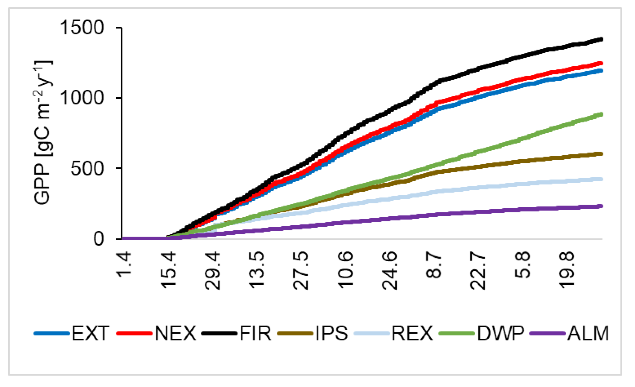
3.2.1. Assimilation (GPP)

Light response curves (LRC) for selected species are shown in Figure S2. Early successional stages species (Calamagrostis villosa, Chamaerion angustifolium, Calamagrostis arundinacea, Salix caprea, Rubus ideaus) showed significantly higher (p < 0.01) values of light saturated GPP (PAR 1500 µmol photons m⁻² s⁻¹ PAR) than shade-tolerant species typical for spruce forests (Picea abies, Vaccinium myrtillus, Avenella flexuosa). The maximum rate of GPP for grasses, herbs and broadleaved trees culminated in late May, while conifers culminated in late June.

GPP_max and α derived from the LRC for seasonal modelling of photosynthesis according to Equation (1) are given in Supplement Table S1. The GPP derived from species-specific LRC was further summarized in 10 cm layers reduced by available PAR and LAI fractions as shown in Figure 4 and calculated for ecosystem types according to vegetation characteristics (LAI and species).

The highest seasonal GPP was fixed in FIR ecosystem type (1,420 ± 33.0 gC m⁻²). Both managed (EXT) and unmanaged (NEX) types assimilated similar amount of C equal to 1198 ± 24.5 and 1250 ± 29.1 gC m⁻² respectively. Dwarf pine fixed 886 ± 17.6 gC m⁻², and spruce forest damaged by bark beetle (IPS) assimilated 605 ± 19.4 gC m⁻². GPP on one-year-old windthrow (REX) and on alpine meadows was 425 ± 16.5 and 230 ± 8.2 g C m⁻², respectively, as presented in Figure 5.

According to the State Forest of TANAP records, the average annual wood stock increment (2012–2013) in Lariceto-Piceetum, prevailing forest community in studied catchments, was 8.0 m³ ha⁻¹ y⁻¹. Using BEF for aboveground (1.3) and belowground spruce biomass (1.2) and CUE (0.35), the estimated GPP was 892 gC m⁻² y⁻¹. If ground vegetation assimilation (330.6 ± 97.8 gC m⁻² y⁻¹) was added, total GPP in undisturbed REF forest was 1222.6 gC m⁻² y⁻¹.

3.2.2. Ecosystem (RE) and Component Respiration

The highest ER was on REF (1148 ± 120.1 gC m⁻² y⁻¹) and IPS (1100 ± 175.0 gC m⁻² y⁻¹), followed by FIR (957 ± 175.0 gC m⁻² y⁻¹) and NEX (909 ± 87.4 gC m⁻²) sites. Soil carbon efflux was the largest component of ecosystem respiration. From all the ecosystem types, the largest annual soil carbon efflux equal to 953 gC m⁻² was in the REF ecosystem. The second largest flux (905 gC m⁻² y⁻¹) was emitted from the IPS type. Soil on the FIR site respired 617 gC m⁻² y⁻¹ and from managed windthrow (EXT) 596 gC m⁻² y⁻¹. Soil respiration from Pinus mugo stands and alpine meadows was equal to 508 and 250 gC m⁻² y⁻¹, respectively.

The average proportion of soil respiration to total ER in studied ecosystems was 74% and ranged from 67% (NEX) to 82% (IPS). Soil respiration showed the highest correlation (avg R² = 0.64) with temperature measured at 10 cm soil depth. The correlation between air temperature and leaf respiration was of similar magnitude (R² = 0.61), while the correlation of air temperature to wood respiration was the lowest (R² = 0.38).

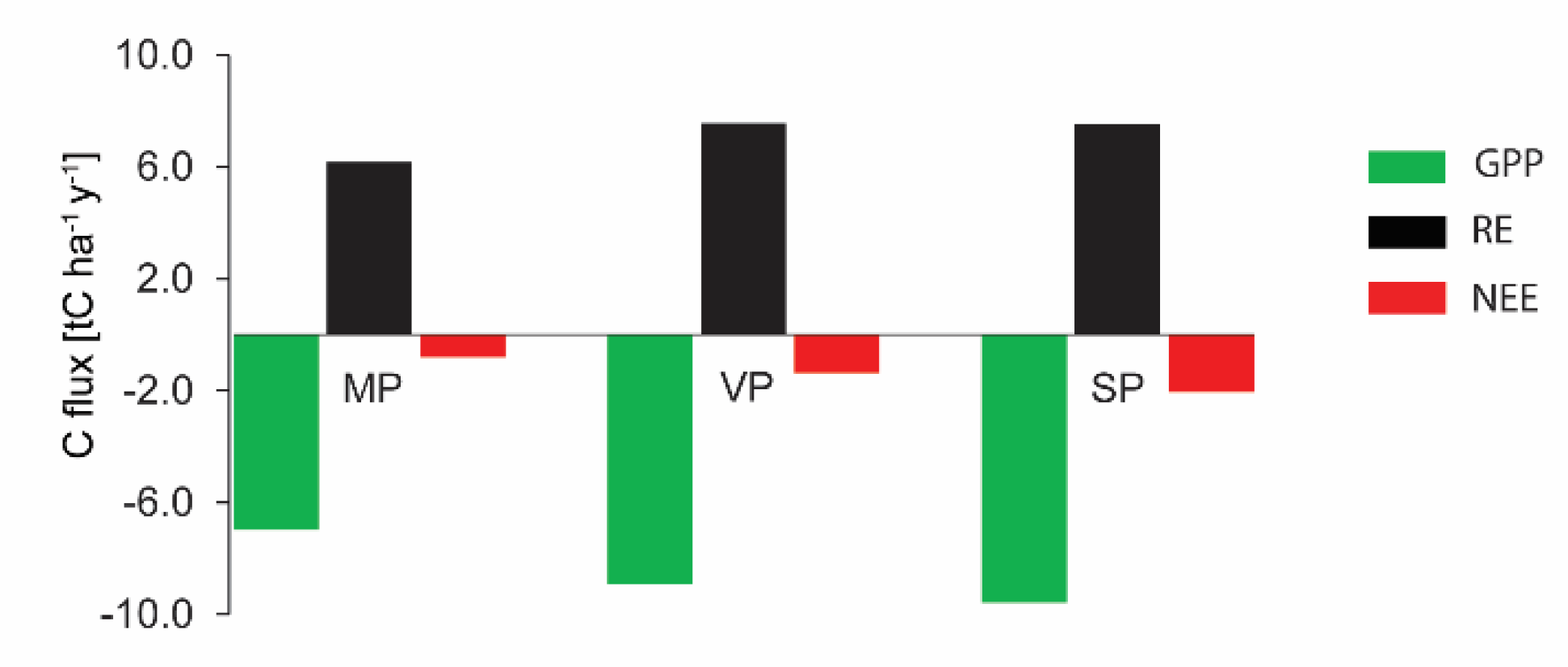
3.2.3. Carbon Balance (NEE)

NEE as a difference between seasonal GPP and annual RE indicates whether the ecosystem or watershed sequesters or emits C to the atmosphere. The GPP, RE and NEE fluxes in the studied ecosystems are presented in

Table 4. Average annual carbon fluxes (gC m⁻² y ⁻¹) and CI (95%) for different ecosystem types.

Flux/ Ecosystem	ALM	DWP	IPS	REF	EXT	FIR	NEX	REX
GPP	−230 ± 8.2	−886 ± 17.6	−605 ± 19.4	−1223 *	−1198 ± 24.5	−1420 ± 33.0	−1250 ± 29.1	−425 ± 16.5
ER	220 ± 43.7	695 ± 90.3	1100 ± 175.0	1148 ± 120.1	846 ± 77.4	957 ± 175.0	909 ± 87.4	755 ± 96.4
NEE	−10 ± 44.5	−191 ± 91.9	495 ± 176.0	−75 ± 120.1	−352 ± 81.2	−463 ± 178.1	−341 ± 92.1	330.0 ± 97.8

* indicates that confidence intervals for the REF were not calculated as a different method was used for GPP estimation.

.

Most of the ecosystems were carbon sink. The largest sink was vegetation on FIR (−463 ± 178.1 gC m⁻² year⁻¹), followed by the EXT and NEX ecosystems. The differences among wind disturbed sites were low mostly due to large variation of SR. Undisturbed mature REF type was carbon neutral (−75 ± 120.1 gC m⁻² year⁻¹, an asterisk indicates that confidence intervals for the REF were not calculated as a different method was used for GPP estimation). IPS was the largest carbon source (495 ± 176 gC m⁻² year⁻¹) followed by one-year-old windthrow REX (330 ± 97.8 gC m⁻² year⁻¹). NEE in IPS and REX remarkably differed from all other ecosystems.

GPP, RE and NEE fluxes (tC ha⁻¹ year⁻¹) in three catchments are presented in Figure 6.

As the GPP and RE increased in order SP > VP > MP, the same order applied for NEE. NEE in MP catchment (−80 ± 73 gC m⁻² y⁻¹) indicates that carbon balance was almost neutral. The VP (−136 ± 84 gC m⁻² y⁻¹) and SP (−206 ± 115 gC m⁻² y⁻¹) acted in 2014 as mild and strong carbon sinks, respectively.

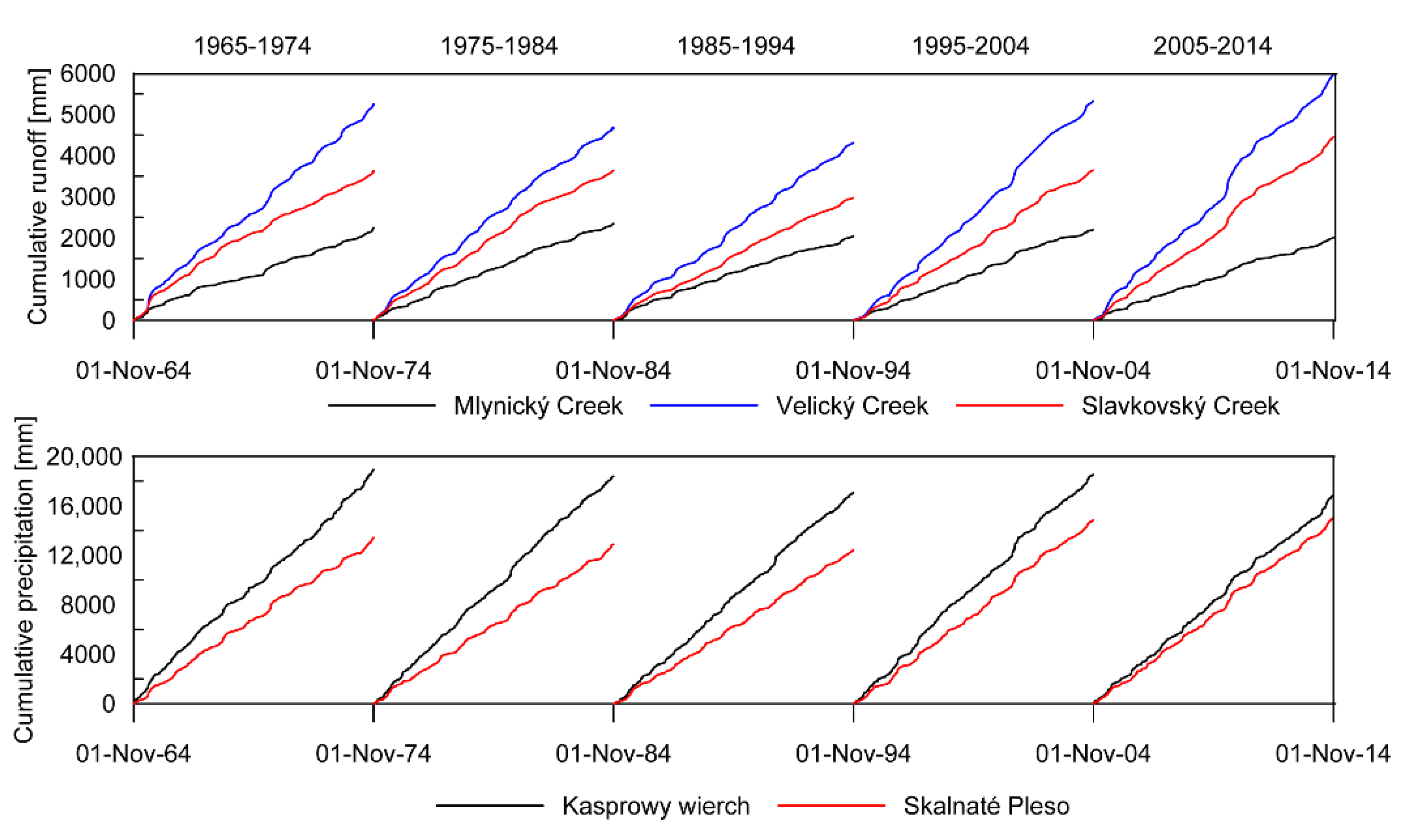
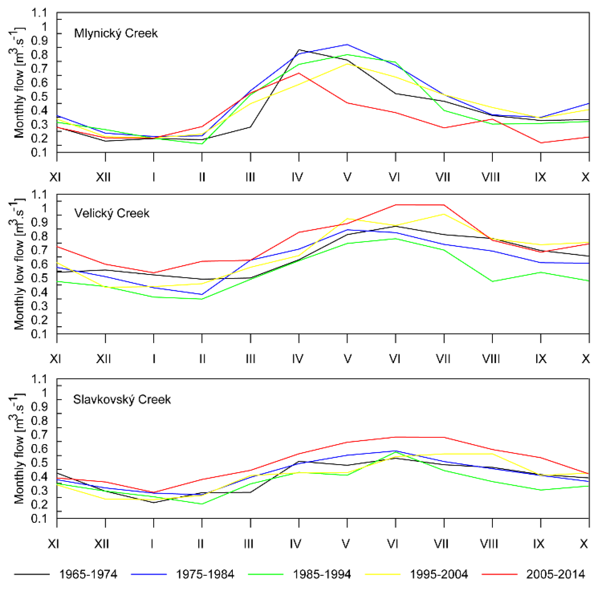
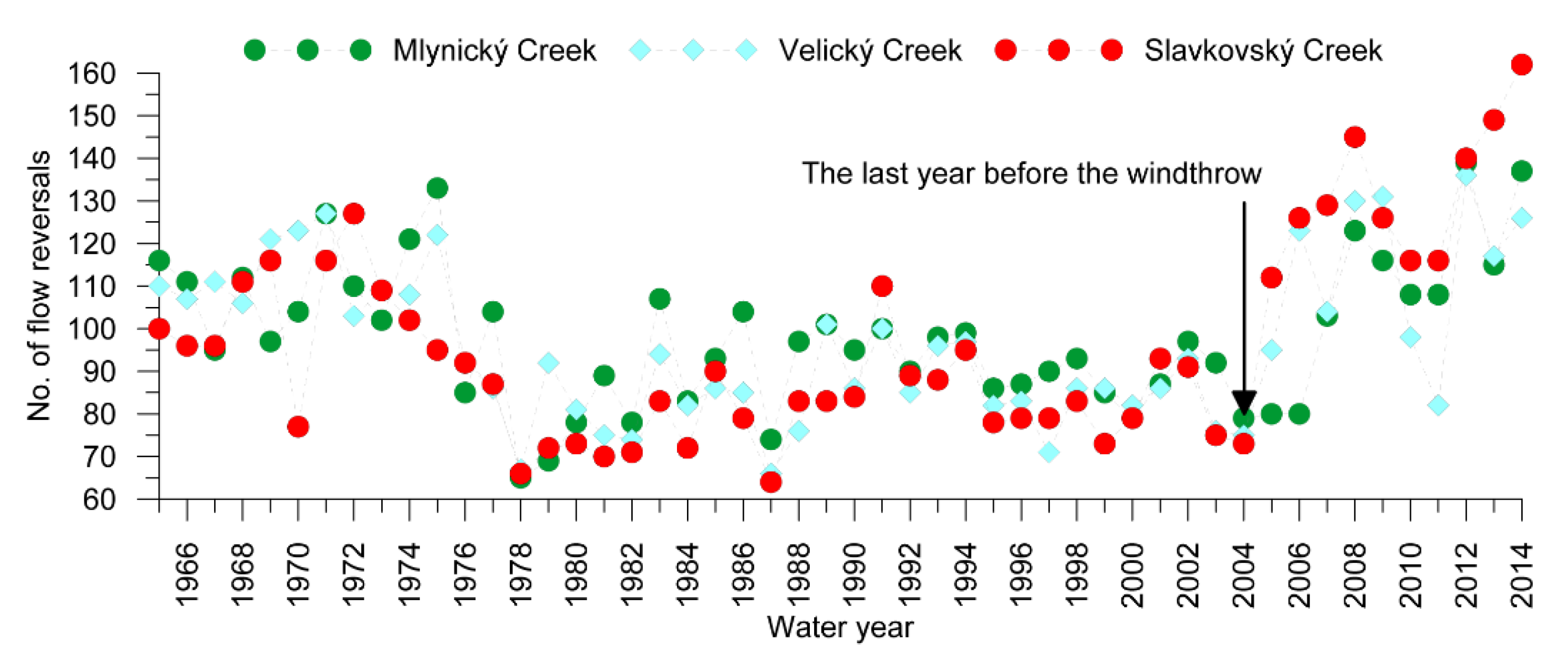
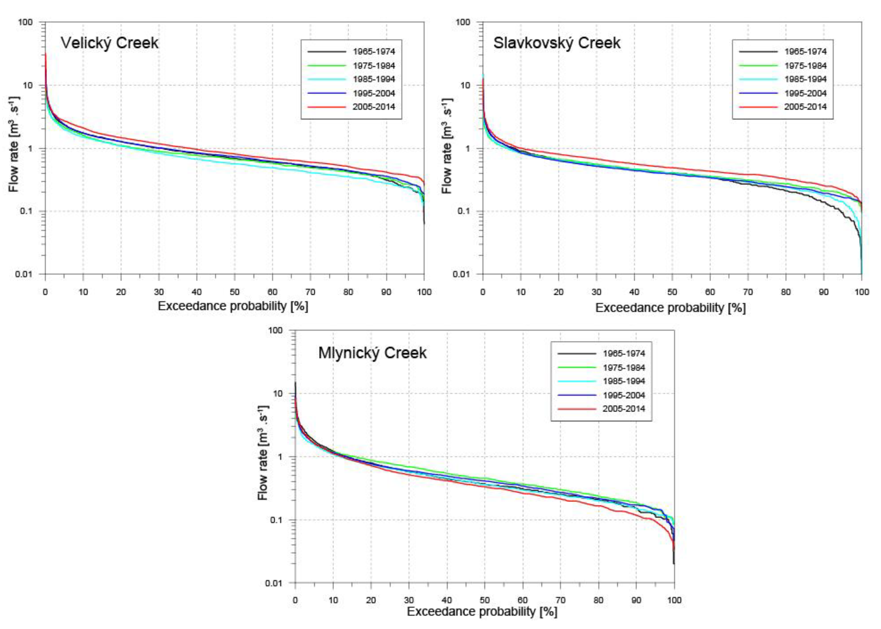
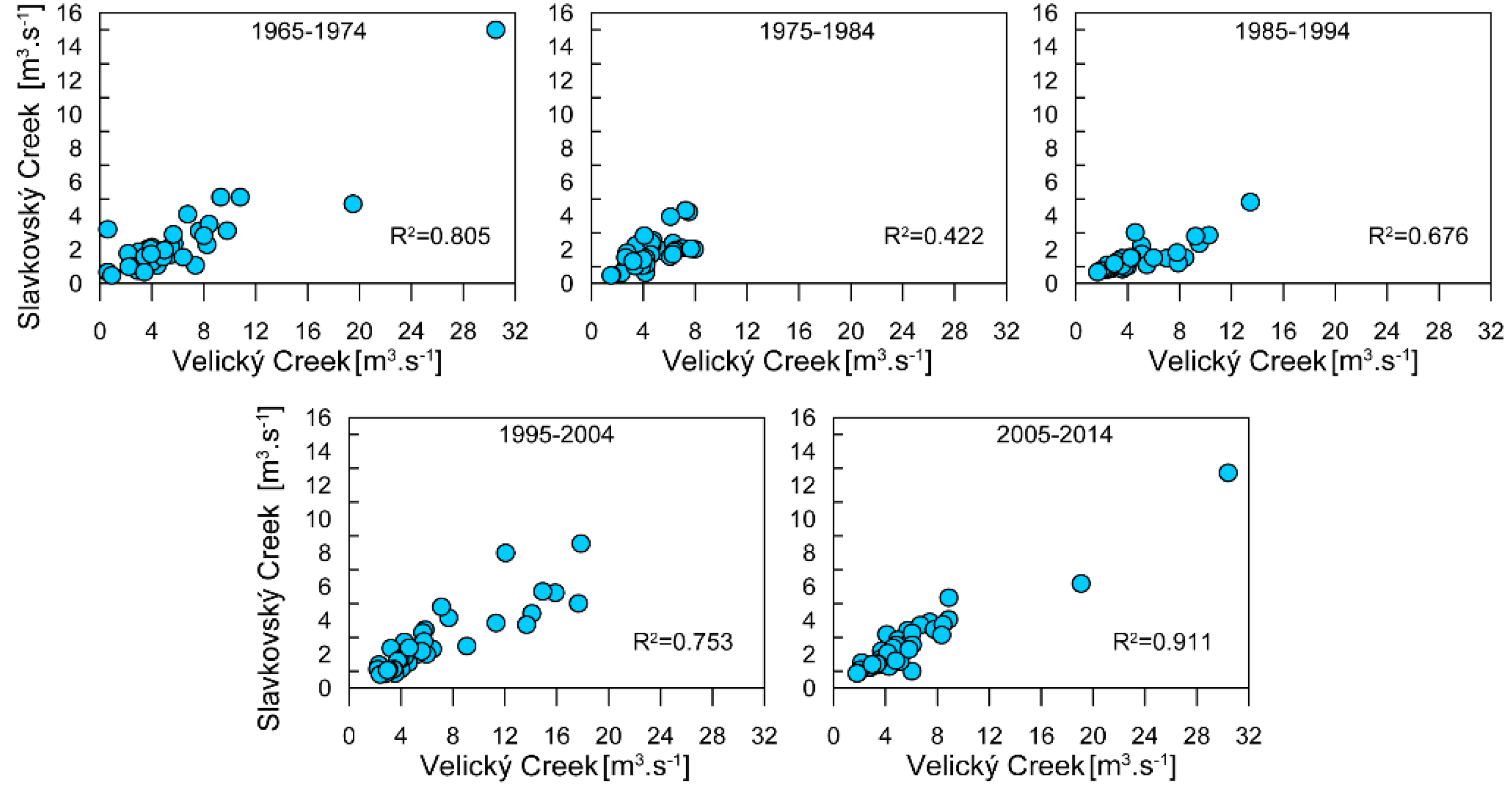
3.3. Streamflow Characteristics

Decadal cumulative precipitation and runoff (Figure 7) revealed greater cumulative runoff in the VP and SP catchments in the decade after the windthrow (2005–2014). Similar increase is not visible in the MP catchment which was very little affected by the windthrow.

Median monthly flows and low flows in the period 2005–2014 increased in almost all months of a year in the SP catchment (Figure 8), while the opposite was observed in the MP catchment in the warm period of a year (May–October), except for August. The smallest changes were found in the VP catchment where they were more pronounced in monthly low flows. Figure 8 also documents seasonal variability of flows in the studied catchments that is probably not related to windthrow. For example, annual maxima in the MP catchment in the 1965–1974 and 2005–2014 decades were clearly related to the snowmelt period (April), while in other decades and other two catchments they occurred later in spring (May, June). A shift in the occurrence of seasonal flow maxima to the summer period (July or even August) is observed in the last two decades (from 1995) of the study period in the VP and SP catchments.

The indicators listed in Table 3 except for the number of flow reversals did not reveal the influence of the disturbances. In water years 2005 and 2006, the number of flow reversals increased in the VP and SP catchments (Figure 9).

Strong increase occurred in the MP catchment in 2007 (interestingly, the number of flow reversals decreased in 2007 in the VP catchment). Variability of this indicator after 2007 became similar in all studied catchments.

In the 2005–2014 decade, flow duration curves (FDCs) in the VP and SP catchments were shifted in the opposite direction compared to the FDC calculated for the MP catchment (Figure 10).

Partial duration peakflow data did not indicate more frequent occurrence of higher discharges. Peakflows of the greatest annual runoff events in the VP and SP creek catchments became better correlated after the disturbance, i.e., in the 2005–2014 decade (Figure 11).

4. Discussion

Forest potential to sequester carbon in biomass and soil and thus to mitigate climate change is of high interest. In reality, a forest, as well as any other vegetation, concurrently fixes and releases carbon. The strength of carbon sink depends on many factors, e.g., species composition, soil properties, age of vegetation, local climate, etc. [62,63]. Disturbances influence forest growth dynamics, mortality and decomposition processes and therefore carbon cycling [64]. Disturbed forests usually become a carbon source, at least temporarily [26,65,66] while disturbed biomass decomposes and productivity decreases. One of the key questions is how long after a disturbance it takes until forest ecosystems recover and become carbon neutral and eventually begin to act as carbon sinks.

Our chamber-based measurements confirmed our expectation that forest ecosystems acted as a carbon source after the disturbance. NEE in the one-year-old windthrow (REX) was 330 gC m⁻² y⁻¹. The 2014 windthrow destroyed dense mature stands with sparse forest floor vegetation which led to strong decline of GPP. Due to canopy destruction also the autotrophic component of ER declined but the impact on NEE was much less pronounced than that on GPP reduction. These data coincide with the EC tower measurements in 2006–2007 [67]. The authors reported strong carbon efflux 2–3 years after the 2004 forest destruction from the same wind-disturbed sites that we analyzed in this paper. Direct measurements of carbon fluxes on windthrown sites are rare, but the impact is often compared to that of logging impact. Rebane et al. [64] in a review of post disturbance carbon balance stated that one year after harvesting the annual efflux usually ranged from 520 to 1000 gC m⁻² y⁻¹ and three years after the disturbance forests emitted 120 gC m⁻² y⁻¹.

Dramatic post disturbance NEE changes were also revealed by our data. We found that ten years after the disturbance the ecosystems affected by the windthrow were either carbon neutral or already became a substantial carbon sink. Niu et al. [14] analyzed the time needed for carbon recovery following different disturbances and pointed out that recovery time was related to disturbance severity with more severe impact requiring longer recovery times. They stated that relatively fast turnover from carbon source to carbon sink was assigned with windthrow (23.5 ± 5 years). The longest recovery time (101 ± 28 years) was needed after wildfires. In our study the burnt site recovered the fastest. The carbon balance estimates at managed, unmanaged and burnt windthrown sites indicate that carbon neutrality was already exceeded in previous years as the NEE values reached −352, −341 and −463 gC m⁻², respectively. Changes in NEE in the years after the disturbance are expected, while their direction and magnitude depend upon the balance between the source effects of the load of decomposing wood [60,68] and the sink effects of the recovering vegetation. Recovery of carbon fluxes after such an extreme windthrow that occurred in the Tatra Mountains, which almost completely destroyed thousands of hectares, was surprisingly fast. Vigorous vegetation recovery on disturbed sites was already reported in our earlier papers [54]. According to Zhu et al. [69], if forest recovery is a dominant mechanism, then the current carbon sink is expected to saturate as forests age and vegetation reaches its late successional stage. This is the very likely future of carbon fate in our study catchments.

The expected difference in carbon balance between the forest that was managed and unmanaged after the disturbance was proven. Despite the fact that EXT exhibited greater species diversity as a consequence of replanting and NEX had more trees [70], the LAI values at the two sites were similar. Removal of undesirable plant species on the EXT site during weed control regularly reduced plant canopy and thus reduced potential carbon sequestration. On the other hand, greater plant diversity, especially of trees on the EXT site, supports forest resilience and future climate change mitigation potential. Dead wood intentionally left on the NEX site has not contributed to ecosystem respiration yet due to still weak decomposition rate of fallen logs. This is the likely reason why our data are in contrast with [71] or [72] who reported higher CO₂ efflux from unmanaged sites than from sites where dead wood was removed.

Contrary to wind disturbed sites, the IPS site acted as a large carbon source in 2015 (NEE = 495 gC m⁻² y⁻¹). Besides reduced assimilation, increased soil respiration was the main factor. Total respiration was the highest at the IPS site from all disturbed sites (1100 gC m⁻² y⁻¹). We attribute this result to elevated heterotrophic respiration. This is in agreement with [73] who reported increased soil respiration after bark beetle outbreak due to elevated microorganism activity stimulated by increased radiation trough open canopy and thus higher soil temperature. According to [64], carbon recovery in a forest disturbed by insects (bark beetles) should be less than 10 years, which is probably not our case. We see the reason for the large carbon efflux in our study in the fact that the studied IPS ecosystems are located outside the reach of downslope winds. Due to less frequent disturbances, the soil is covered with thicker humus horizons and thus contains more carbon. More light, elevated temperature and moisture stimulate more intensive decomposition and carbon efflux. Higher content of organic compounds in soil as well as less evident pit and mound microtopography indicate that the forest that is currently attacked by the bark beetles was rarely affected by the disturbances in the past [74]. On the other hand, [75] reported respiration decline after a bark beetle attack. They found decreasing carbon input from assimilation more important for forest carbon balance than increasing respiration of dead material. Regardless, large stock of labile carbon poses a risk of carbon release to the atmosphere under climatic warming [13,76]. Soil temperature was identified as a key environmental factor for respiration on wind-disturbed sites. The highest correlation was with soil respiration, the weakest with stem respiration. Don et al. [77] reported increased soil temperature by 4 °C and higher decomposition rates on the bare soil just after the disturbance in the Tatra Mountains compared to the intact forest. Fast decaying fine material (needles, bark) after the bark beetle attack probably also supported the increase of heterotrophic respiration, as stated by [11]. Heterotrophic respiration could also profit from increased soil moisture because of suppressed tree transpiration. Although ten years after the disturbance soil moisture did not notably differ between the disturbed and intact forest stands, it played only a marginal role in soil respiration rate. We suppose that sufficient soil moisture (around 30% Θ_vol) during the entire study period has not limited respiration.

Carbon sequestration on wind-disturbed sites massively exceeded the performance of the intact mature Norway spruce forest (−75 ± 120 gC m⁻² y⁻¹). Higher carbon sequestration in post-disturbance forests is rather common. For example, [14] showed primary productivity higher by 35% than the pre-disturbance values. In our study, the post-disturbance carbon sequestration was three times higher than before forest destruction. Nevertheless, intact forest NEE values must be interpreted with caution. The NPP and consequently the GPP flux were estimated by the biometric method, while in other ecosystem types they were estimated by gasometrical methods. Calculated NEE values were much lower than those reported for comparable temperate forests. Intact forests in central Europe are generally expected to act as a carbon sink [78,79]. According to [10], European forests potentially sequester carbon from −115 to −410 gC m⁻². Etzold et al. [80] reported −153 gC m⁻² y⁻¹ from comparable Norway spruce stands in the Alps. Thus, the performance of mature forests in our study can be classified as carbon neutral, rather than a small sink. One of the possible explanations for low NPP production in our study might be less intense growth of mature trees. Mean annual increment of spruce forests in central Europe is 14 m³ ha⁻¹ [10]. At our study sites it reached only 8 m³ ha⁻¹ per year. It is obvious that NEE declines with age [81]. Direct measurements using eddy covariance method showed that middle age stands are stronger carbon sinks than very old stands [64,82]. However, forest age is not the case in our study as observed trees are 80−120 years old and the explanation of small GPP and NEE requires further analysis.

Upscaling of CO₂ fluxes from leaf to ecosystem/landscape scales is always challenging. However, it is necessary because quantification of source and sink relationships at a landscape level is inevitable to understand the relationships between NEE and the global carbon cycle [83]. Cleary et al. [27] compared leaf versus ecosystem fluxes in a grass-dominated ecosystem and found higher NEE with a leaf measurement. NEE declined in whole plant chambers reported [84] as a consequence of self-shading. Occasionally, the authors found twofold greater GPP_max in sparse than in dense populations. In our study we found similar differences between GPP measured by Licor XT6400 at a leaf scale versus whole plant in the closed chamber. Leaf-scale measurement yielded on average 50% higher GPP values unless empirical models for vertical LAI distribution and PAR dissipation were applied. After the correction, the difference declined below 12%. We applied this correction in GPP calculation when the LAI exceeded 2.5 m² m⁻² and the shading effect became evident.

The analysis of streamflow characteristics did not unambiguously indicate the influence of forest disturbances. Only a few characteristics exhibited different behavior after the disturbances. Greater cumulative runoff in the most severely affected VP and SP catchments in 2005–2014 decade could be related to the disturbances. Górnik et al. [85] documented an increase in the number of days with precipitation of 40–60 mm in the warm period of the year (May–October) since 2001 and the unusually wet year 2010 was observed in the Tatra Mountains. Greater cumulative decadal runoff compared to the 1975–1984 and 1985–1994 decades occurred also before the windthrow, i.e., in the decade 1995–2004. However, the values calculated for the VP and SP catchments at the end of 2005–2014 decade exceeded analogical values from all previous decades. This was not observed in the MP catchment with forest cover almost unaffected by the windthrow. Cumulative point precipitation at the end of the decade 2005–2014 is not greater than in the previous four decades. These data indicate the influence of forest disturbances. On the other hand, Figure 7 shows that the greatest increase in cumulative runoff occurred approximately between April and December 2010 and another significant increase was observed since April 2014, i.e., about five and nine years after the windthrow. The winters of 2010 and 2014 were both exceptionally snow-poor [86] and summer 2010 was very wet. It is therefore possible that the increased runoff after the snow-poor winters was related more to the snowmelt-precipitation regime in springs 2010 and 2014 than to the effects of forest disturbances.

The number of flow reversals is another indicator that increased in the VP and SP catchments in the years following the windthrow while it remained stable in the MP catchment in 2005 and 2006. Although the MP catchment was very little affected by the windthrow, a strong increase in the number of flow reversals was observed in 2007 (Figure 9). This could be related to massive forest dieback and following cutting. It is worth noting that greater numbers of flow reversals occurred also in the 1960s although some values after the windthrow were greater. The highest values that occurred in the SP catchment in 2013 and 2014 are probably not related to the windthrow. Because the variability of the indicator is similar in all studied catchment has been similar since 2008, we assume that the high values in 2012–2014 were caused by meteorological causes rather than by forest disturbances.

Although median decadal flow duration curves in the VP and SP catchments after the windthrow are slightly shifted to greater discharges at almost all probabilities of occurrence, our earlier analysis of the annual FDCs indicated that the shift was probably not caused solely by the disturbances, but also by meteorological conditions in the years 2005, 2010 and 2014 [48]. Similarly, higher correlations among peakflow discharges in the VP and SP catchments in the 2005–2014 period (Figure 11) were more influenced by meteorological conditions than by the effects of forest disturbances. Greater ranges of measured peak discharges given by higher precipitation (e.g., in June 2010) resulted in higher coefficients of determination between the discharges in the neighboring catchments of the Velický and Slavkovský Creek.

5. Conclusions

Our study revealed that ten years after extremely severe disturbances, the carbon balance at a catchment scale was neutral or even positive. Highest carbon sequestration occurred at the most heavily disturbed sites. Positive carbon balance reflects very intensive growth of successional vegetation in recent warm and sufficiently moist climate. Only small patches of the forest killed by bark beetle acted as a carbon source. Both managed and unmanaged sites in our study catchments acted as carbon sinks. Nevertheless, greater species diversity on the managed sites could potentially guarantee higher forest resilience and climate change mitigation effect under future, hardly predictable, conditions. The findings that the intact mature forest was carbon neutral requires further and more detailed study to identify the reasons.

Possible reasons for unclear effects of the disturbances on catchment hydrology were suggested by [45]. Most of the forest damage, while quite extensive, occurred in the middle sections of the catchments. The headwater areas, where most of the runoff is formed and where little forest existed before anyway, were not damaged by the windthrow. Windthrow deforested areas were built by moraines with high infiltration capacity. This disturbance affected relatively smaller percentages of catchment areas since it hit the catchments in the east-western direction, while the catchments are generally north-south oriented. Thus, not all the forests were damaged by the windthrow (although the subsequent disturbances in the SP catchment destroyed 98% of the original forests). Additional analyses conducted in this article confirm our previous conclusion about the lack of suitable indicators of changes in catchment hydrology in headwater mountain catchments with areas of several tens of square kilometers in which the forest disturbances affected up to 20–32% of the catchment area.

References

1. Thom, D.; Seidl, R. Natural disturbance impacts on ecosystem services and biodiversity in temperate and boreal forests. Biol. Rev. 2015, 91, 760–781. [Google Scholar] [CrossRef] [PubMed]
2. Senf, C.; Seidl, R. Mapping the coupled human and natural disturbance regimes of Europe’s forests. BioRxiv 2020. [Google Scholar] [CrossRef] [Green Version]
3. Seidl, R.; Schelhaas, M.J.; Lexer, M.J. Unraveling the drivers of intensifying forest disturbance regimes in Europe. Glob. Chang. Biol. 2011, 17, 2842–2852. [Google Scholar] [CrossRef]
4. Anderegg, W.R.L.; Kane, J.M.; Anderegg, L.D.L. Consequences of widespread tree mortality triggered by drought and temperature stress. Nat. Clim. Chang. 2013, 3, 30–36. [Google Scholar] [CrossRef]
5. Malhi, Y.; Franklin, J.; Seddon, N.; Solan, M.; Turner, M.G.; Field, C.B.; Knowlton, N. Climate change and ecosystems: Threats, opportunities and solutions. Philos. Trans. R. Soc. B 2020, 375. [Google Scholar] [CrossRef] [Green Version]
6. Weiskopf, S.R.; Rubenstein, M.A.; Crozier, L.G.; Gaichas, S.; Griffis, R.; Halofsky, J.E.; Hyde, K.J.W.; Morelli, T.L.; Morisette, J.T.; Muñoz, R.C.; et al. Climate change effects on biodiversity, ecosystems, ecosystem services, and natural resource management in the United States. Sci. Total Environ. 2020, 733. [Google Scholar] [CrossRef]
7. IPCC. Climate Change 2013: The Physical Science Basis. In Contribution of Working Group I to the Fifth Assessment Report of the Intergovernmental Panel on Climate Change; IPCC: Geneva, Switzerland, 2013. [Google Scholar]
8. Perdrial, J.; Brooks, P.D.; Swetnam, T.; Lohse, K.A.; Rasmussen, C.; Litvak, M.; Harpold, A.A.; Zapata-Rios, X.; Broxton, P.; Mitra, B.; et al. A net ecosystem carbon budget for snow dominated forested headwater catchments: Linking water and carbon fluxes to critical zone carbon storage. Biogeochemistry 2018, 138, 225–243. [Google Scholar] [CrossRef]
9. Bellassen, V.; Luyssaert, S. Managing forests in uncertain times. Nature 2014, 506, 153–155. [Google Scholar] [CrossRef] [Green Version]
10. Nabuurs, G.; Schelhaas, M. Carbon profiles of typical forest types across Europe assessed with CO2FIX. Ecol. Indic 2002, 1, 213–223. [Google Scholar] [CrossRef]
11. Harmon, M.E.; Bond-Lamberty, B.; Tang, J.; Vargas, R. Heterotrophic respiration in disturbed forests: A review with examples from North America. J. Geophys. Res. Biogeosci. 2011, 116, 1–17. [Google Scholar] [CrossRef]
12. Amiro, B.D.; Barr, A.G.; Barr, J.G.; Black, T.A.; Bracho, R.; Brown, M.; Chen, J.; Clark, K.L.; Davis, K.J.; Desai, A.R.; et al. Ecosystem carbon dioxide fluxes after disturbance in forests of North America. J. Geophys. Res. 2010, 115, G00K02. [Google Scholar] [CrossRef]
13. Kurz, W.A.; Dymond, C.G.; Stinson, G.J.; Rampley, G.J.; Neilson, E.T.; Carroll, A.L.; Ebata, T.; Safranyik, L. Mountain pine beetle and forest carbon feedback to climate change. Nature 2008, 452, 987–990. [Google Scholar] [CrossRef] [PubMed]
14. Niu, S.; Fu, Z.; Luo, Y.; Stoy, P.C.; Keenan, T.F.; Poulter, B.; Zhang, L.; Piao, S.; Zhou, X.; Zheng, H.; et al. Interannual variability of ecosystem carbon exchange: From observation to prediction. Glob. Ecol. Biogeogr. 2017, 26, 1225–1237. [Google Scholar] [CrossRef]
15. Calderón-Loor, M.; Cuesta, F.; Pinto, E.; Gosling, W.D. Carbon sequestration rates indicate ecosystem recovery following human disturbance in the equatorial Andes. PLoS ONE 2020, 15, e0230612. [Google Scholar] [CrossRef] [PubMed]
16. Anderegg, W.R.L.; Martinez-Vilalta, J.; Cailleret, M.; Camarero, J.J.; Ewers, B.E.; Galbraith, D.; Gessler, A.; Grote, R.; Huang, C.; Levick, S.R.; et al. When a Tree Dies in the Forest: Scaling Climate-Driven Tree Mortality to Ecosystem Water and Carbon Fluxes. Ecosystems 2016, 19, 1133–1147. [Google Scholar] [CrossRef] [Green Version]
17. Levy-Varon, J.H.; Schuster, W.S.F.; Griffin, K.L. Rapid rebound of soil respiration following partial stand disturbance by tree girdling in a temperate deciduous forest. Oecologia 2014, 174, 1415–1424. [Google Scholar] [CrossRef]
18. Seidl, R.; Schelhaas, M.; Rammer, W.; Verkerk, P. Increasing forest disturbances in Europe and their impact on carbon storage. Nat. Clim. Chang. 2014, 4, 806–810. [Google Scholar] [CrossRef] [Green Version]
19. Reichstein, M.; Bahn, M.; Ciais, P.; Frank, D.; Mahecha, M.D.; Senevirante, S.I.; Zscheischler, J.; Beer, C.; Buchmann, N.; Frank, D.C.; et al. Climate extremes and the carbon cycle. Nature 2013, 500, 287–295. [Google Scholar] [CrossRef]
20. Hlásny, T.; Barcza, Z.; Fabrika, M.; Balász, B.; Churkina, G.; Pajtík, J.; Sedmák, R.; Turčáni, M. Climate change impacts on growth and carbon balance of forests in Central Europe. Clim. Res. 2011, 47, 219–236. [Google Scholar] [CrossRef] [Green Version]
21. Pugh, T.A.M.; Arneth, A.; Kautz, M.; Poulter, B.; Smith, B. Important role of forest disturbances in the global biomass turnover and carbon sinks. Nat. Geosci. 2019, 12, 730–735. [Google Scholar] [CrossRef]
22. Klein, D.; Höllerl, S.; Blaschke, M.; Schulz, C. The contribution of managed and unmanaged forests to climate change mitigation-A model approach at stand level for the main tree species in Bavaria. Forests 2013, 4, 43–69. [Google Scholar] [CrossRef]
23. Moore, P.T.; DeRose, R.J.; Long, J.N.; van Miegroet, H. Using Silviculture to Influence Carbon Sequestration in Southern Appalachian Spruce-Fir Forests. Forests 2012, 3, 300–316. [Google Scholar] [CrossRef]
24. Baldocchi, D.D. Assessing the eddy covariance technique for evaluating carbon dioxide exchange rates of ecosystems: Past, present and future. Glob. Chang. Biol. 2003, 9, 479–492. [Google Scholar] [CrossRef] [Green Version]
25. Noe, S.M.; Kimmel, V.; Hüve, K.; Copolovici, L.; Portillo-Estrada, M.; Püttsepp, Ü.; Jõgiste, K.; Niinemets, Ü.; Hörtnagl, L.; Wohlfahrt, G. Ecosystem-scale biosphere-atmosphere interactions of a hemiboreal mixed forest stand at Järvselja, Estonia. For. Ecol. Manag. 2011, 262, 71–81. [Google Scholar] [CrossRef] [Green Version]
26. Lindauer, M.; Schmid, H.P.; Grote, R.; Mauder, M.; Steinbrecher, R.; Wolpert, B. Net ecosystem exchange over a non-cleared wind-throw-disturbed upland spruce forest—Measurements and simulations. Agric. For. Meteorol. 2014, 197, 219–234. [Google Scholar] [CrossRef]
27. Cleary, M.B.; Naithani, K.J.; Ewers, B.E.; Pendall, E. Upscaling CO2 fluxes using leaf, soil and chamber measurements across successional growth stages in a sagebrush steppe ecosystem. J. Arid. Environ. 2015, 121, 43–51. [Google Scholar] [CrossRef]
28. Wang, K.; Liu, C.; Zheng, X.; Pihlatie, M.; Li, B.; Haapanala, S.; Vesala, T.; Liu, H.; Wang, Y.; Liu, G.; et al. Comparison between eddy covariance and automatic chamber techniques for measuring net ecosystem exchange of carbon dioxide in cotton and wheat fields. Biogeosciences 2013, 10, 6865–6877. [Google Scholar] [CrossRef] [Green Version]
29. Luo, X.; Chen, J.M.; Liu, J.; Black, T.A.; Croft, H.; Staebler, R.; McCaughey, H. Comparison of big-leaf, two-big-leaf, and two-leaf upscaling schemes for evapotranspiration estimation using coupled carbon-water modeling. J. Geophys. Res. Biogeosci. 2018, 123, 207–225. [Google Scholar] [CrossRef]
30. Kostka, Z.; Holko, L. Role of forest in hydrological cycle—Forest and runoff. Meteorol. J. 2006, 9, 143–148. [Google Scholar]
31. Andreassian, V. Waters and forests: From historical controversy to scientific debate. J. Hydrol. 2004, 291, 1–27. [Google Scholar] [CrossRef]
32. Ben-Hur, M.; Fernandez, C.; Sakkola, S.; Santamarta-Cerezal, J.C. Overland flow, soil erosion and stream water quality in forest under diferent pertubations and climate conditions. In Forest Management and Water Cycle; Bredemeier, M., Cohen, S., Godbold, D., Lode, E., Pichler, V., Eds.; Springer: Berlin/Heidelberg, Germany, 2011; pp. 263–289. [Google Scholar]
33. Bartík, M.; Holko, L.; Jančo, M.; Škvarenina, J.; Danko, M.; Kostka, Z. Influence of mountain spruce forest dieback on snow accumulation and melt. J. Hydrol. Hydromech. 2019, 67, 59–69. [Google Scholar] [CrossRef] [Green Version]
34. Bosch, J.M.; Hewlett, J.D. A review of catchment ex-periments to determine the effect of vegetation changes on water yield and evapotranspiration. J. Hydrol. 1982, 55, 3–23. [Google Scholar] [CrossRef]
35. Best, A.; Zhang, L.; McMahon, T.; Western, A.; Vertessy, R. A Critical Review of Paired Catchment Studies with Reference to Seasonal Flows and Climatic Variability. In CSIRO Land and Water Technical Report 25/03; Murray Darling Basin Commission: Canberra, Australia, 2003; p. 56. ISBN 1 876 830 57 3. [Google Scholar]
36. Jones, J.A.; Post, D.A. Seasonal and successional streamflow response to forest cutting and regrowth in the northwestern and eastern United States. Water Res. 2004, 40, W05203. [Google Scholar] [CrossRef]
37. Stednick, J.D. Monitoring the effects of timber harvest on annual water yield. J. Hydrol. 1996, 176, 79–95. [Google Scholar] [CrossRef]
38. Alila, Y.; Kuraś, P.K.; Schnorbus, M.; Hudson, R. Forests and floods: A new paradigm sheds light on age-old controversies. Water Resour. Res. 2009, 45, W08416. [Google Scholar] [CrossRef]
39. The Nature Conservancy. Indicators of Hydrologic Alteration Version 7.1 User’s Manual. Nat. Conserv. 2009. Available online: https://www.conservationgateway.org/Files/Pages/indicators-hydrologic-altaspx47.aspx (accessed on 1 March 2014).
40. Olden, J.D.; Poff, N.L. Redundancy and the choice of hydrologic indices for characterizing streamflow regimes. River Res. Appl. 2003, 19, 101–121. [Google Scholar] [CrossRef]
41. Gao, Y.; Vogel, R.M.; Kroll, C.N.; Olden, J.D. Development of representative indicators of hydrologic alteration. J. Hydrol. 2009, 374, 136–147. [Google Scholar] [CrossRef]
42. Vogel, R.M.; Sieber, J.; Archfield, S.A.; Smith, M.P.; Apse, C.D.; Huber-Lee, A. Relations among storage, yield, and instream flow. Water Resour. Res. 2007, 43, W05403. [Google Scholar] [CrossRef]
43. Holeksa, J.; Zielonka, T.; Zywiec, M.; Fleischer, P. Identifying the disturbance history over a large area of larch-spruce mountain forest in Central Europe. For. Ecol. Manag. 2016, 361, 318–327. [Google Scholar] [CrossRef]
44. Fleischer, P.; Homolová, Z. Long-term ecological research in larch-spruce forest community after natural disturbances in the Tatra Mts. Lesn. Cas. For. J. 2011, 57, 237–250. [Google Scholar]
45. Holko, L.; Fleischer, P.; Novák, V.; Kostka, Z.; Bičárová, S.; Novák, J. Hydrological Effects of a Large Scale Windfall Degradation in the High Tatra Mountains, Slovakia. In Management of Mountain Watersheds; Křeček, J., Haigh, M., Hofer, T., Kubin, E., Eds.; Springer: Berlin/Heidelberg, Germany, 2012; pp. 164–179. [Google Scholar]
46. Holko, L.; Hlavatá, H.; Kostka, Z.; Novák, J. Hydrological regimes of small catchments in the High Tatra Mountains before and after extraordinary wind-induced deforestation. Folia Geogr. Ser. Geogr. Phys. 2009, 15, 33–44. [Google Scholar]
47. Holko, L.; Kostka, Z.; Novák, J. Estimation of groundwater recharge, water balance of small catchments in the High Tatra Mountains in hydrological year 2008. In Sustainable Development and Bioclimate: Reviewed Conference Proceedings; Pribullová, A., Bičárová, S., Eds.; Geophysical Institute of the Slovak Academy of Sciences: Bratislava, Slovakia, 2009; pp. 93–94. [Google Scholar]
48. Holko, L.; Škoda, P. Assessment of runoff changes in selected catchments of the High Tatra Mountains ten years after the windthrow. Acta Hydrolog. Slovaca 2016, 17, 43–50. (In Slovak) [Google Scholar]
49. Rasband, W.S. Image J. U.S. National Institutes of Health, Bethesda, Maryland, USA. Available online: https://imagej.nih.gov/ij/ (accessed on 30 September 2015).
50. Pajtík, J.; Konôpka, B.; Lukac, M. Biomass functions and expansion factors in young Norway spruce (Picea abies [L.] Karst) trees. For. Ecol. Manag. 2008, 256, 1096–1103. [Google Scholar] [CrossRef]
51. Pajtík, J.; Konôpka, B.; Bošela, M.; Šebeň, V.; Kaštier, P. Modelling forage potential for red deer: A case study in post-disturbance young stands of rowan. Ann. For. Res. 2015, 58, 91–107. [Google Scholar] [CrossRef] [Green Version]
52. Pajtík, J.; Konôpka, B.; Šebeň, V.; Michelčík, P.; Fleischer, P. Biomass allocation of common larch in the first age class in the High Tatra Mts. Stud. Tatra Natl. Park. 2015, 44, 237–249. [Google Scholar]
53. Pajtík, J.; Konôpka, B. Quantifying edible biomass on young Salix caprea and Sorbus aucuparia trees for Cervus elaphus: Estimates by regression models. Austrian J. For. Sci. 2015, 132, 61–80. [Google Scholar]
54. Fleischer, P.; Fleischer, P., Jr.; Gömöryová, E.; Celer, S. Upscaling carbon fluxes from chamber measurement to the landscape-scale in spruce forest disturbed by windthrow in the Tatra Mts. In Landscape and Landscape Ecology, Proceedings of the 17th int symposium on Landscape Ecology; Halada, L., Bača, A., Boltižiar, M., Eds.; Institute of Landscape Ecology, Slovak Academy of Sciences: Nitra, Slovakia, 2016; pp. 227–235. [Google Scholar]
55. Drewitt, G.B.; Black, T.A.; Nesic, Z.; Humphreys, E.R.; Jork, E.M.; Swanson, R.; Ethier, G.J.; Griffis, T.; Morgenstern, K. Measuring forest floor CO2 fluxes in a Douglas-fir forest. Agric. For. Meteorol. 2002, 110, 299–317. [Google Scholar] [CrossRef]
56. Fleischer, P.; Fleischer, P., Jr.; Celer, S. Carbon balance in spruce forest affected by wind and insect disturbances in the Tatra Mts: Methodological approach and preliminary results. In Aktuálne Problémy v Ochrane Lesa; Kunca, A., Ed.; National Forest Center: Zvolen, Slovakia, 2013; pp. 113–120. (In Slovak) [Google Scholar]
57. Marek, M.V. Carbon in Ecosystems under Changing Climate in Czech Republic; Academia Praha: Prague, Czech Repulic, 2011. (In Czech) [Google Scholar]
58. Ryan, M.G.; Lavigne, M.B.; Gower, S.T. Annual carbon cost of autotrophic respiration in boreal forest ecosystems in relation to species and climate. J. Geophys. Res. 1997, 102, 28871–28883. [Google Scholar] [CrossRef] [Green Version]
59. Buchmann, N. Biotic and abiotic factors controlling soil respiration rates in Picea abies stands. Soil. Biol. Biochem. 2000, 32, 1625–1635. [Google Scholar] [CrossRef]
60. Knohl, A.; Søe, A.R.B.; Kutsch, W.L.; Göckede, M.; Buchmann, N. Representative estimates of soil and ecosystem respiration in an old beech forest. Plant Soil 2008, 302, 189–202. [Google Scholar] [CrossRef] [Green Version]
61. Searsy, J.K. Flow-Duration Curves; Geological Survey Water-Supply-Papet 1542-a: Washington, DC, USA, 1959; p. 33. [Google Scholar]
62. Curtis, P.S.; Gough, C.M. Forest aging, disturbance and the carbon cycle. N. Phytol. 2018, 219, 1188–1193. [Google Scholar] [CrossRef] [PubMed] [Green Version]
63. Yuan, J.; Jose, S.; Hu, Z.; Pang, J.; Hou, L.; Zhang, S. Biometric and eddy covariance methods for examining the carbon balance of a larix principis-rupprechtii forest in the Qinling Mountains, China. Forests 2018, 9, 67. [Google Scholar] [CrossRef] [Green Version]
64. Rebane, S.; Jõgiste, K.; Kiviste, A.; Stanturf, J.A.; Metslaid, M. Patterns of carbon sequestration in a young forest ecosystem after clear-cutting. Forests 2020, 11, 126. [Google Scholar] [CrossRef] [Green Version]
65. Amiro, B.D.; Barr, A.G.; Black, T.A.; Iwashita, H.; Kljun, N.; McCaughey, H.; Morgenstern, K.; Murayama, S.; Nesic, Z.; Orchansky, A.L.; et al. Carbon, energy and water fluxes at mature and disturbed forest sites, Saskatchewan, Canada. Agric. For. Meteorol. 2006, 136, 237–251. [Google Scholar] [CrossRef]
66. Lindroth, A.; Lagergren, F.; Grelle, A.; Klemedtsson, L.; Langvall, O.; Weslien, P.; Tuulik, J. Storms can cause Europe-wide reduction in forest carbon sink. Glob. Chang. Biol. 2009, 15, 346–355. [Google Scholar] [CrossRef]
67. Giorgi, S.; Fleischer, P.; Gioli, B.; Kolle, O.; Manca, G.; Matese, A.; Zaldei, A.; Ziegler, W.; Cescatti, A.; Miglietta, F.; et al. Carbon Dioxide Fluxes of a Recent Large Windthrow in the High Tatra. Abstract of CEIP Conference. Sissi-Lassithi, Crete. 2006. Available online: http://carboeurope.org/ceip/conference/abstacts/VU_poster/Giorgi) (accessed on 1 November 2006).
68. Lindroth, A.; Grelle, A.; Morén, A.S. Long-term measurements of boreal forest carbon balance reveal large temperature sensitivity. Glob. Chang. Biol. 1998, 4, 443–450. [Google Scholar] [CrossRef]
69. Zhu, K.; Zhang, J.; Niu, S.; Chu, C.; Luo, Y. Limits to growrh of forest biomass carbon sink under climate change. Nat. Commun. 2020. [Google Scholar] [CrossRef] [Green Version]
70. Michalová, Z.; Morrissey, R.C.; Wohlgemuth, T.; Bače, R.; Fleischer, P.; Svoboda, M. Salvage-Logging after Windstorm Leads to Structural and Functional Homogenization of Understory Layer and Delayed Spruce Tree Recovery in Tatra Mts., Slovakia. Forests 2017, 8, 88. [Google Scholar] [CrossRef] [Green Version]
71. Pumpanen, J.; Westman, C.J.; Ilvesniemi, H. Soil CO2 efflux from a podzolic forest soil before and after forest clear-cutting and site preparation. Boreal Environ. Res. 2004, 9, 199–212. [Google Scholar]
72. Koster, K.; Puttsepp, U.; Pumpanen, J. Comparison of soil CO2 flux between uncleared and cleared windthrow areas in Estonia and Latvia. For. Ecol. Manag. 2011, 262, 65–70. [Google Scholar] [CrossRef]
73. Morehouse, K.; Johns, T.; Kaye, J.; Kaye, M. Carbon and nitrogen cycling immediately following bark beetle outbreaks in southwestern ponderosa pine forests. For. Ecol. Manag. 2008, 255, 2698–2708. [Google Scholar] [CrossRef]
74. Fleischer, P.; Koreň, M. Selected forest soil properties after the 2004 windfall in the Tatra Mts. In Sustainable Development and Bioclimate; Pribullová, A., Bičarová, S., Eds.; Geophysical Institute of the Slovak Academy of Sciences: Bratislava, Slovakia, 2009; pp. 77–78. [Google Scholar]
75. Moore, D.J.P.; Trahan, N.A.; Wilkes, P.; Quaife, T.; Stephens, B.B.; Elder, K.; Desai, A.R.; Negron, J.; Monson, R.K. Persistent reduced ecosystem respiration after insect disturbance in high elevation forests. Ecol. Lett. 2013, 16, 731–737. [Google Scholar] [CrossRef] [PubMed] [Green Version]
76. Hagedorn, F.; Mulder, J.; Jandl, R. Mountain soils under a changing climate and land-use. Biogeochemistry 2010, 97, 1–5. [Google Scholar] [CrossRef] [Green Version]
77. Don, A.; Bärwolff, M.; Kalbitz, K.; Andruschkewitsch, R.; Jungkunst, H.F.; Schulze, E.D. No rapid soil carbon loss after a windthrow event in the High Tatra. For. Ecol. Manag. 2012, 276, 239–246. [Google Scholar] [CrossRef]
78. Valentini, R. EUROFLUX: An integrated network for studying the long-term responses of biospheric exchanges of carbon, water, and energy of European forests. Fluxes Carbon. Water Energy Eur. For. 2003, 163, 1–8. [Google Scholar]
79. Grünwald, T.; Bernhofer, C. A decade of carbon, water and energy flux measurements of an old spruce forest at the Anchor Station Tharandt. Tellus Ser. B Chem. Phys. Meteorol. 2007, 59, 387–396. [Google Scholar] [CrossRef] [Green Version]
80. Etzold, S.; Ruehr, N.K.; Zweifel, R.; Dobbertin, M.; Zingg, A.; Pluess, P.; Häsler, R.; Eugster, W.; Buchmann, N. The Carbon Balance of Two Contrasting Mountain Forest Ecosystems in Switzerland: Similar Annual Trends, but Seasonal Differences. Ecosystems 2011, 14, 1289–1309. [Google Scholar] [CrossRef]
81. Taylor, A.R.; Seedre, M.; Brassard, B.W.; Chen, H.Y.H. Decline in Net Ecosystem Productivity Following Canopy Transition to Late-Succession Forests. Ecosystems 2014, 17, 778–791. [Google Scholar] [CrossRef]
82. Luyssaert, S.; Schulze, E.D.; Börner, A.; Knohl, A.; Hessenmöller, D.; Law, B.E.; Ciais, P.; Grace, J. Old-growth forests as global carbon sinks. Nature 2008, 455, 213–215. [Google Scholar] [CrossRef]
83. Yi, C.; Li, R.; Wolbeck, J.; Xu, X.; Nilsson, M.; Aires, L.; Albertson, J.D.; Ammann, C.; Arain, M.A.; De Araujo, A.C.; et al. Climate control of terrestrial carbon exchange across biomes and continents. Environ. Res. Lett. 2010, 5. [Google Scholar] [CrossRef]
84. Kulmala, L.; Pumpane, J.; Hari, P.; Vesala, T. Photosynthesis of ground vegetation in different aged pine forests: Effect of environmental factors predicted with a process-based model. J. Veg. Sci. 2011, 22, 96–110. [Google Scholar] [CrossRef]
85. Górnik, M.; Holko, L.; Pociask-Karteczka, J.; Bičárová, S. Varibility of precipitation and runoff in the entire High Tatra Mountains in the period 1961–2010. Prace Geograficzne 2017, 151, 53–74. [Google Scholar] [CrossRef] [Green Version]
86. Holko, L.; Sleziak, P.; Danko, M.; Bičárová, S.; Pociask-Karteczka, J. Analysis of changes in hydrological cycle of a pristine mountain catchment. 1. Water balance components and snow cover. J. Hydrol. Hydromech. 2020, 68, 180–191. [Google Scholar] [CrossRef]
Figure 1. Ecosystem types (legend in Table 1) in the carbon study part of the catchments; MP (area to stream gage 83 km2, mean altitude 991 m a.s.l., mean slope 9.2°), VP (area 58 km2, mean altitude 1094 m a.s.l., mean slope 9.3°) and SP (area 43 km2, mean altitude 1017 m a.s.l., mean slope 8.6°).
Water 12 02917 g001
Figure 2. Total leaf area index (LAI) (m2 m−2) and species share [%] for ecosystem types on disturbed sites, where NEX—non-extracted windthrow, FIR—burnt windthrow, EXT—extracted windthrow, IPS—forest killed by bark beetle, REX—one-year-old extracted windthrow.
Water 12 02917 g002
Figure 3. Seasonal changes of LAI on ten-year-old windthrow, between May and August 2014; the dots represent means from 25 plots, and the whiskers show SD.
Water 12 02917 g003
Figure 4. Relative distribution of LAI (a) and PAR dissipation (b) in relation to relative canopy depth; black dots—average values for all measured species, line-fitted model.
Water 12 02917 g004
Figure 5. Seasonal (April 1–August 31) sum of GPP for studied ecosystem types, where EXT—extracted windthrow, NEX—non-extracted windthrow, FIR—burnt windthrow, IPS—forest killed by bark beetle, REX—extracted one-year-old windthrow, DWP—dwarf pine, ALM—alpine meadow.
Water 12 02917 g005
Figure 6. Annual carbon fluxes (tC ha−1 y−1) on a catchment scale where MP—Mlynický Creek catchment, VP—Velický Creek catchment, SP—Slavkovský Creek catchment, green bars—GPP, black bars—RE and red bars—NEE. Negative values of NEE indicate carbon sink.
Water 12 02917 g006
Figure 7. Cumulative runoff and precipitation in decades from 1965–1974 to 2004–2014; precipitation data adopted from Holko et al., 2020.
Water 12 02917 g007
Figure 8. Medians of monthly flow characteristics observed in the decades from 1965–1974 to 2005–2014.
Water 12 02917 g008
Figure 9. Number of flow reversals per year in the study catchments; the windthrow occurred at the beginning of the water year 2005.
Water 12 02917 g009
Figure 10. Median decadal flow duration curves.
Water 12 02917 g010
Figure 11. Relationships between peakflow discharges (four greatest runoff events in each year) in the VP (horizontal axis) and SP (vertical axis) catchments in the decades from 1965–1974 to 2005–2014.
Water 12 02917 g011