An Empirical Orthogonal Function-Based Approach for Spatially- and Temporally-Extensive Soil Moisture Data Combination


1
College of Resources and Environmental Engineering, Ludong University, Yantai 264025, China
2
Department of Ecosystem Science and Management, Pennsylvania State University, University Park, PA 16802, USA
3
Grassland Research Institute, Chinese Academy of Agricultural Sciences, Huhhot 010010, China
4
State Key Laboratory of Soil and Sustainable Agriculture, Institute of Soil Science, Chinese Academy of Sciences, Nanjing 210008, China
5
Research Center for Eco-Environment Sciences, Chinese Academy of Sciences, Beijing 100085, China
6
Department of Environmental Science and Technology, University of Maryland, College Park, MD 20742, USA
*
Authors to whom correspondence should be addressed.
Water 2020, 12(10), 2919; https://doi.org/10.3390/w12102919
Submission received: 15 September 2020
/
Revised: 15 October 2020
/
Accepted: 16 October 2020
/
Published: 19 October 2020
(This article belongs to the Special Issue Advanced Technologies and Methods for Soil Water Monitoring and Management)
Abstract
:Modeling and prediction of soil hydrologic processes require identifying soil moisture spatial-temporal patterns and effective methods allowing the data observations to be used across different spatial and temporal scales. This work presents a methodology for combining spatially- and temporally-extensive soil moisture datasets obtained in the Shale Hills Critical Zone Observatory (CZO) from 2004 to 2010. The soil moisture was investigated based on Empirical Orthogonal Function (EOF) analysis. The dominant soil moisture patterns were derived and further correlated with the soil-terrain attributes in the study area. The EOF analyses indicated that one or two EOFs of soil moisture could explain 76–89% of data variation. The primary EOF pattern had high values clustered in the valley region and, conversely, low values located in the sloping hills, with a depth-dependent correlation to which curvature, depth to bedrock, and topographic wetness index at the intermediate depths (0.4 m) exhibited the highest contributions. We suggest a novel approach to integrating the spatially-extensive manually measured datasets with the temporally-extensive automatically monitored datasets. Given the data accessibility, the current data merging framework has provided the methodology for the coupling of the mapped and monitored soil moisture datasets, as well as the conceptual coupling of slow and fast pedologic and hydrologic functions. This successful coupling implies that a combination of diverse and extensive moisture data has provided a solution of data use efficiency and, thus, exciting insights into the understanding of hydrological processes at multiple scales.
1. Introduction
Soil moisture is a crucial variable within earth system dynamics from regional to pedon scales [1,2]. Identification and prediction of soil moisture patterns are essential in a wide range of agronomic, hydrological, pedological, and environmental studies [3,4]. However, it is challenging to obtain accurate information on soil moisture at appropriate temporal and spatial scales [5,6]. This shortage of information has impeded the modeling, prediction, and management of water resources [7,8,9,10]. Linking soil moisture mapping with monitoring can provide a more integrated approach to amplify the information on soil moisture in understanding soils and water resources [11,12,13] and provides a way of combatting the general decline of field hydrology relative to modeling [14].
Previous studies have indicated that the spatial pattern of soil moisture is highly dependent on various controlling factors such as parent material, soil, land use/vegetation, topography, and climate [1,8,15,16]. However, separating the relative importance of each factor is usually tricky as some of the influencing factors are interdependent due to the scale-dependence, dry-wet cycles, and interface exchange from top to deep soil layers [1,15,17,18]. During wet conditions, the subsurface lateral flow may be necessary, whereas, during dry conditions, the vertical surface flow at the onset of precipitation has more influence [8,11]. The correlation length of soil moisture ranges from near zero to a thousand meters. It is highly dependent on both the study scale and the measurement density [19], with an exact direct proportionality of increasing correlation lengths with increasing scales having been observed. For on-site soil moisture monitoring system or networks, the correlation measurements typically include several sites. In contrast, for the measurements characterizing soil moisture variation within the field, the area can cover several ha, or even larger sizes for satellite-based investigations [20]. The potential exists for more accurate estimation of soil moisture by using synergistic approaches among various earth observation methodologies.
The procedures for associating the relatively stable spatial patterns of soil moisture and specific soil hydrologic processes with precipitation events are sorely lacking. The temporal variations related to field measurements of soil moisture have been displayed in numerous studies that have shown that terrain-derived indices rarely explained >50% of soil moisture variability [1,15,16]. Although climate seasonality and localized vs. non-local hydrological fluxes usually exert a strong influence on surface soil moisture distribution [8,15,21], less is understood regarding the subsurface soil moisture spatial patterns. By integrating spatially-distributed soil, topographical and meteorological data, Schwärzel et al. [22] developed an integrated ecological approach, which provided a more accurate description of soil moisture variability than the traditional mapping. Other research using a modification of this approach showed that both spatial distribution and temporal evolution of soil moisture might be investigated at multiple scales [23]. Another potential improvement consists of integrating geophysical scanning with real-time soil moisture monitoring [24,25]. Real-time soil moisture monitoring may provide information concerning actual hydrologic dynamics and the timing of preferential flow occurrence. At the same time, geophysical scans may verify the spatial distribution of preferential flow pathways. The synthesis of these methods may enhance data accuracy and associated processes, thus increasing our understanding of hydrological processes in various soils and landscapes [20,24].
Spatial dependency is commonly characterized and quantified by geostatistical methods, such as autocorrelation and semi-variogram analysis [18,26]. An additional approach to analyze the spatial patterns of soil moisture and their relationships with controlling factors is through an empirical orthogonal function (EOF) analysis [27,28]. EOF analysis decomposes a dataset into a series of orthogonal spatial patterns. These underlying (stable) patterns may be correlated with variables derived from topography, soil, vegetation, land management, and meteorology to identify the most important tendencies of the soil moisture. Yoo and Kim [29] investigated the spatial and temporal variability of field-scale soil moisture. They concluded that no unique and straightforward mechanism could be applied to explain the evolution of the soil moisture field. Wagenet [30] summarized the main factors influencing soil moisture from the pore scale to the global scale and recognized soil and topography as essential local controls of soil moisture variations. During dry periods, soil moisture distribution may be conceptualized as being controlled predominantly by soil properties, whereas during wet periods, the topography is the controlling factor within a landscape. However, the plot scale results have not been easily transferable to hillslope and catchment scales. Theoretical and empirical approaches have been used to quantify hydrological dynamics based on such ‘point-scale’ data that tends to over- or underestimate parameters and fluxes [31]. There are still not enough data points in time nor in space to characterize these controlling processes, given substantial temporal and spatial variability [20].
Usually, while the temporal frequency for the manual measurement of soil moisture with more points is approximately weekly-or monthly-based, the automated monitoring data may be hourly-based or daily-based but with less spatial coverage [2]. It might be a viable cost-efficient alternative to combine data sets with different spatial and temporal resolutions for a complicated landscape [32]. Martinez et al. [33] used the approach of combining datasets to investigate soil moisture dynamics and patterns in a small catchment in Australia, where 500 datapoints were sampled weekly for four weeks, together with seven continuously measuring stations. In their study, high-resolution soil moisture data combining manual measurements at irregular time intervals provided a valuable addition to the time series of precipitation and discharge to investigate runoff generation. However, it is lacking in the complete merging of data.
In this study, part of our soil moisture dataset contains manually measured data that offers better spatial coverage of many sites, but with limited temporal frequency, as only weekly measurements were made. Another part of our soil moisture dataset contains automatically monitored data that offers better temporal frequency with repetitive ten-min to one-hour measurements but only limited spatial coverage with a limited number of selected sites. It is expected that the product of this combination will capture the temporal dynamics of soil moisture from the automatically monitored data and with improved spatial variation using the information from manual measurements. The objectives of this study were to: (1) assess the dominant soil moisture spatial-temporal patterns based on multi-year datasets; (2) determine how these patterns are controlled by terrain, soil, and vegetation as a function of scale, wetness, and depth; and (3) provide a possible way to integrate spatial-extensive datasets with temporal-extensive datasets.
2. Materials and Methods
2.1. Study Area
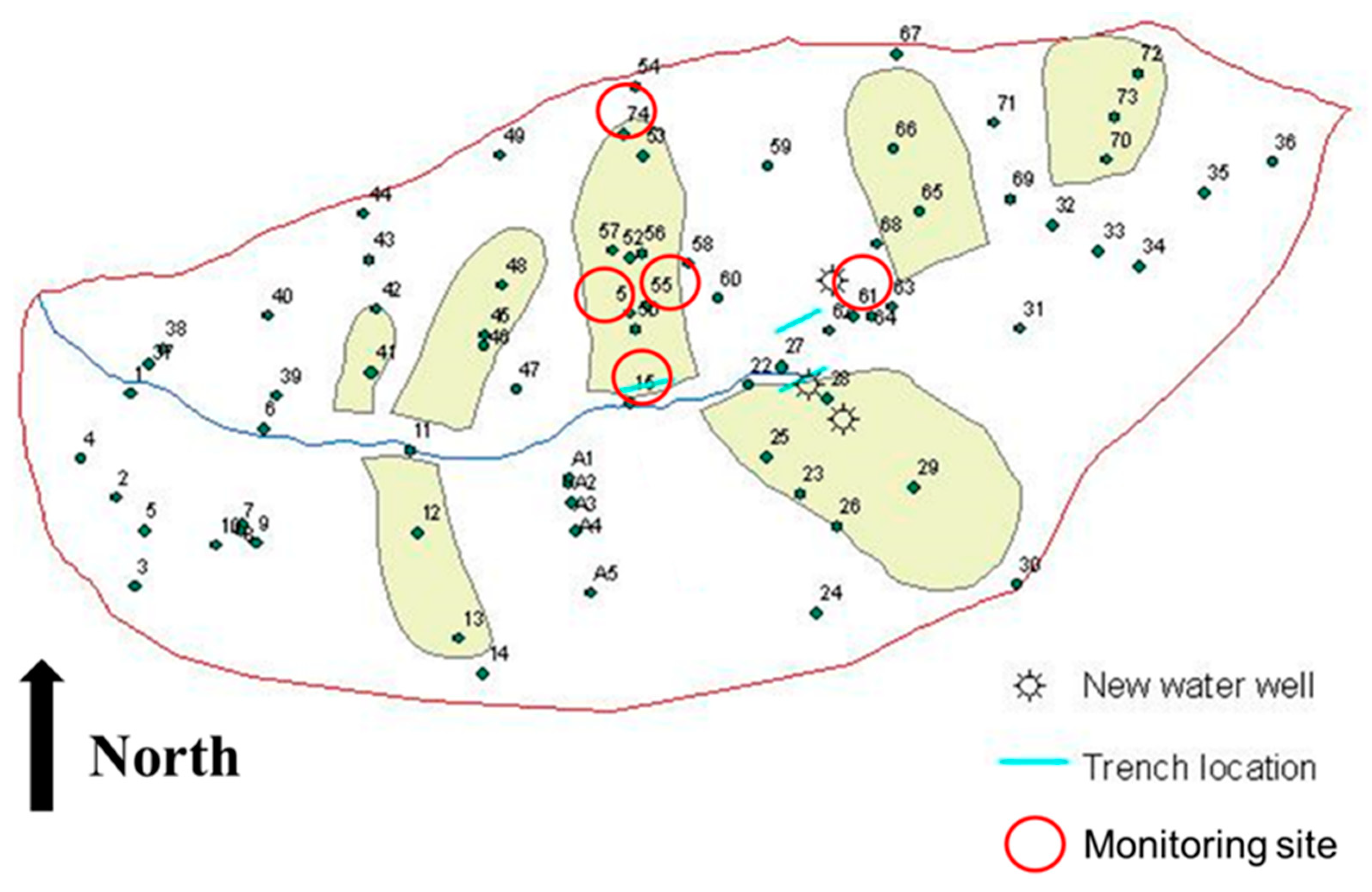
The forested Shale Hills catchment has an area of 7.9-ha and is located in Huntingdon County, PA, on the eastern coast of the USA. The catchment is V-shaped, with a first-order stream in the valley and moderately steep slopes on both sides (Figure 1). Swales are inter-dispersed within the catchment, five and two swales on the south- and north-facing slope, respectively. Elevation ranges from 256 m at the catchment outlet to 310 m at the ridge. The catchment is underlain by about 300-m thick, medium-dark gray to olive-colored, steeply bedded, highly fractured Rose Hill Shale that exhibits reddish-brown iron oxidation stains [6]. Depth to bedrock ranges from <0.25 m on the ridgetop and upper side slopes to >2–3 m on the valley floor and swales. The soils were developed from shale colluvium or residuum, with many channery shale fragments. Five soil series were identified according to the USDA classification in different landscape units [34]: (1) the Weikert series, a shallow, well-drained soil on the steep planar or convex hillslopes and summit regions; (2) the Berks series, a moderately deep, well-drained soil on the toe-slope positions and side-slopes of concave hillslopes; (3) the Rushtown series, a deep, moderately well-drained soil in concave hillslopes and some other parts of the catchment; (4) the Earnest series, a very deep, poorly-drained soil in the valley bottoms and near a stream zone; and (5) the Blairton series, a deep, poorly to moderately-drained soil within the valley bottom at the east portion of the catchment [6]. The area has a typical humid continental climate with mean monthly minimum temperatures of −3 °C in January and a maximum of 22 °C in July (National Weather Service, State College, PA, USA). The annual precipitation is about 980 mm and is roughly evenly distributed throughout the year, with high intensity, short-duration storm events during the summer convective rainfall.
2.2. Data Collection
At the Shale Hills Catchment, a total of 106 manual soil moisture measurement locations were recorded weekly over a 6-yr period (2004 to 2010; Figure 1). We used a portable TRIME-T3 time domain reflectometry (TDR) Tube Probe (IMKO, Ettlingen, Germany) to determine soil moisture contents (m3 m−3) using a 0.051-m diameter PVC access tube installed at each sampling site at a specific depth (i.e., 0.1-, 0.2-, 0.4-, 0.6-, 0.8-, and 1.0-m). Soil moisture storage was calculated by the measured water content, multiplying its corresponding depth. The measurement accuracy of the 0.2 m-long TRIME-T3 probe is ±2.0% in the range of 0 to 40% and ±3.0% in 40% to 60% for most soils. Two or three readings were taken in orthogonal directions (probe rotated 90° between measurements), and the mean value was used. Before each round of measurement, the probe was calibrated in the laboratory with glass beads with known moisture content. However, soil horizon specific calibration was not taken due to the diversity of soils in the catchment and the large number of sites monitored [6]. The number of locations measured on each measurement day varied due to the number of actual places, personnel availability, and weather conditions. The subsequent analysis includes 36 days where at least 65 soil moisture annual measurement locations were measured, as a trade-off between having a sufficient number of measuring sites for an adequate spatial coverage and sufficient sampling days for a complete temporal range covering different season/wetness conditions. Among these 36 measurement days were 13 wets (>22%), 14 moist (<22%, >15%), and 9 dries (<15%), respectively, based on the field averaged wetness condition.
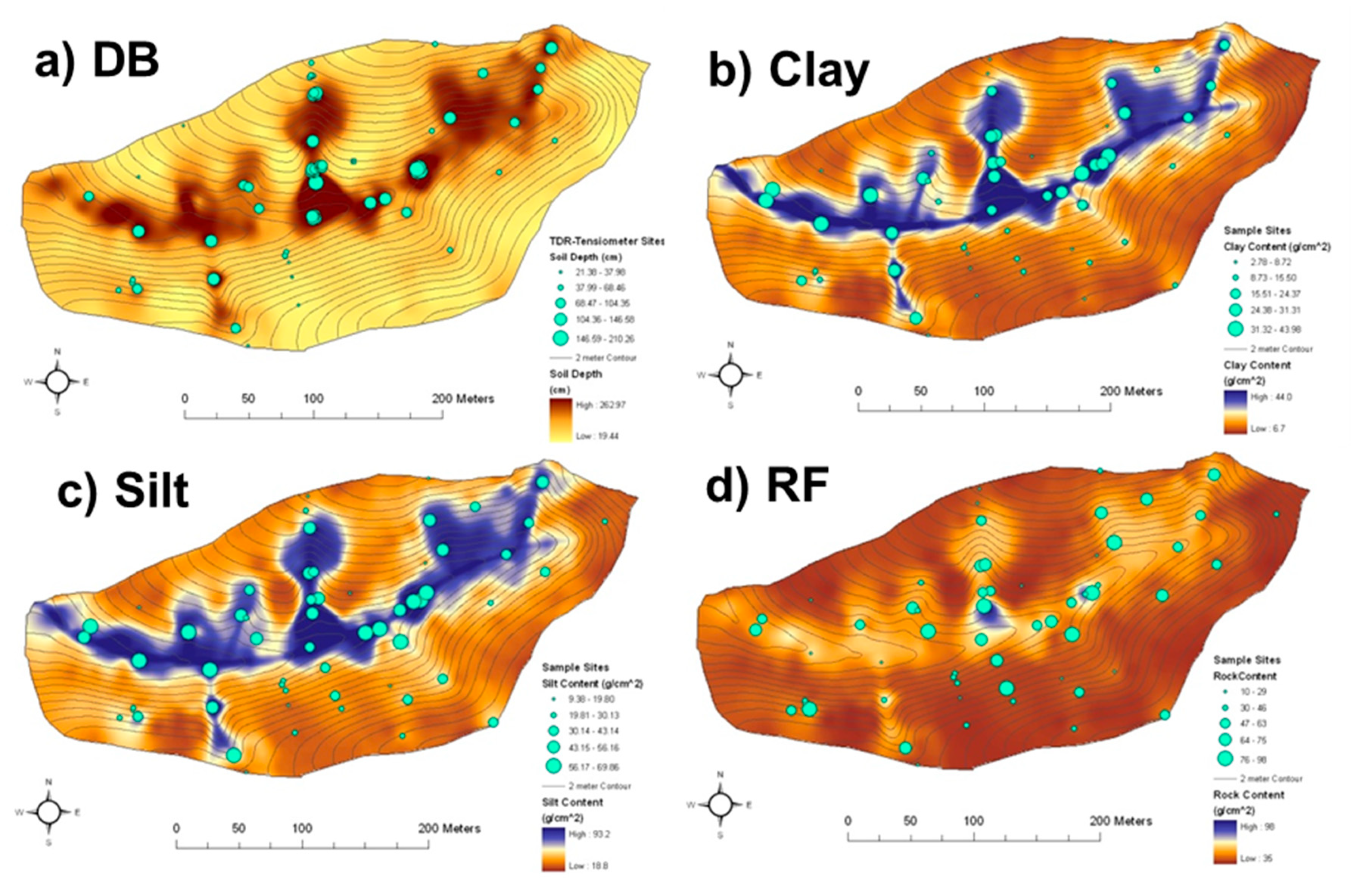
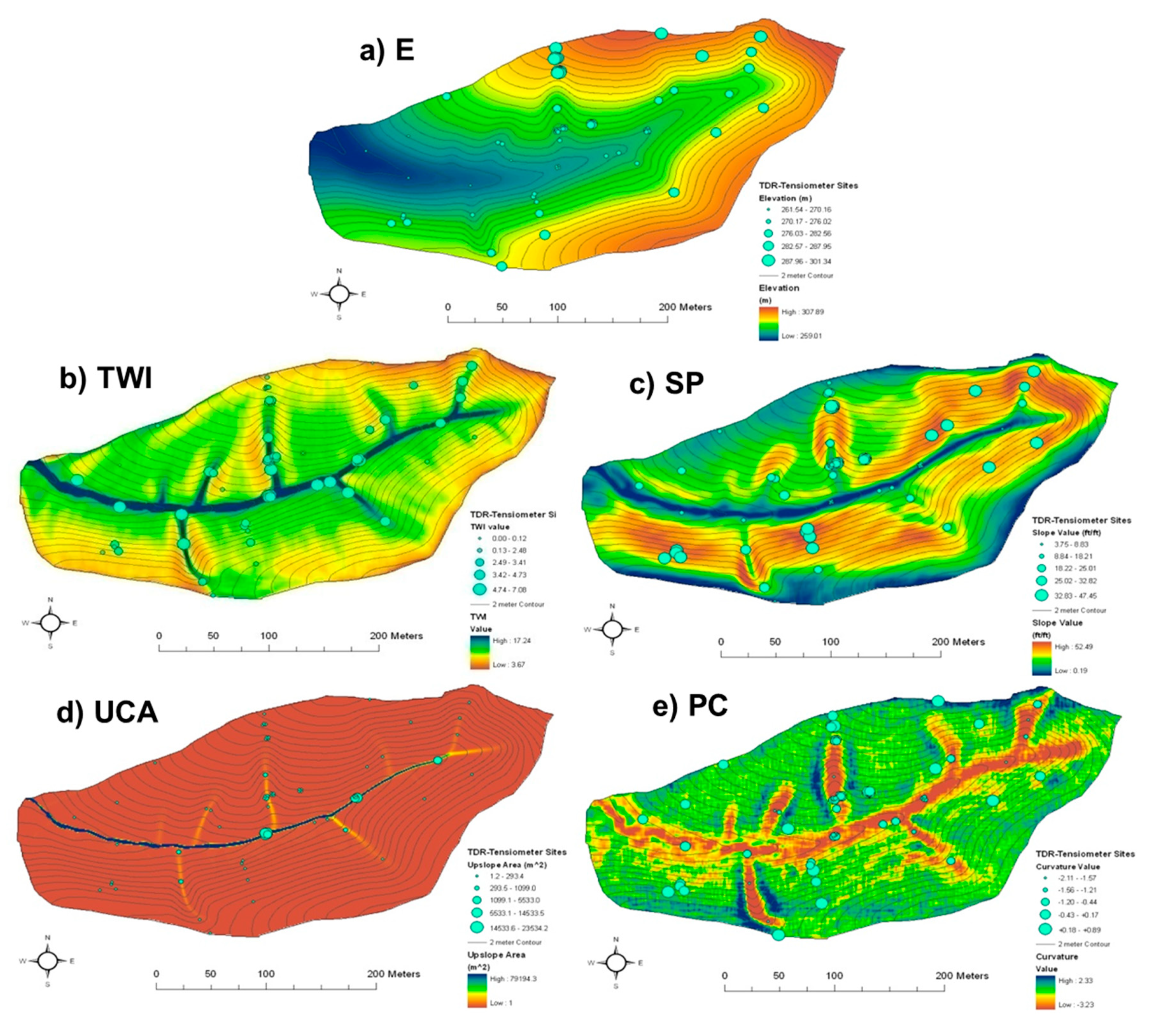
At each sampling site of soil water content, intact soil cores were collected to characterize other properties that influence water patterns and dynamics. In particular, using standard soil survey procedures [6], we firstly described each soil core, including thickness, horizon, texture, structure, and rock fragment (Figure 2). Before performing soil textural analysis, rock fragments (defined as soil particles that did not pass through a 2-mm sieve) were separated from the bulk sample and weighed to determine the percentage rock fragment in each horizon. Depth to bedrock (varying from <0.5 m along the planar hillslopes to >2 m along the valley floor) was determined from 223 point-based observations during soil mapping and monitoring tube installation using a handheld auger. A digital elevation model (DEM) of the catchment was interpolated from light detecting and ranging (LiDAR) elevation point clouds collected by an airplane flown over the catchment (PAMAP, PA Department of Conservation and Natural Resources). About 40,000 LiDAR elevation points were converted into a 1 × 1 m2 DEM using ArcGIS 9.2 (ESRI Inc., Redland, CA, USA). The smoothed DEM was then used to derive the terrain attributes such as elevation, slope, curvature, upslope contributing area, and topographic wetness index at all soil moisture annual measurement and monitoring locations (Figure 3). Maps of soil properties were interpolated using regression kriging, which combines linear regression modeling between a target variable and auxiliary variable(s) with simple kriging of the model residuals, in order to predict the value of the target variable at unmeasured locations, due to the complex landscape structure and also the accessibility of spatially exhaustive auxiliary variables such as variables derived from DEM [6,20]. To assess how well the regression kriging predicted target variable at unmeasured locations, we performed a leave-one-out cross validation that removed one measurement location, and used regression kriging based on the remaining measurement locations to predict target variable at the missing location. We calculated root mean squared error (RMSE) and coefficients of determination (R2) to assess the reliability of the estimate.
In addition to manual measurement, soil moisture was monitored in real-time (with a temporal resolution of 5 s) at five representative sites (one for each soil series), at different depths at each location depending on soil thickness and horizon. These sites are located from the ridge top (site 74; Weikert series) to the valley bottom (site 61; Ernest series), with both planar (site 51; Rushtown series)/convex (site 53; Berks series) hillslopes and concave swales (site 15; Blairton series) (Figure 1). At each long-term monitoring site, a pit was excavated, and capacitance-type probes from Decagon Devices, Pullman WA (EC10 or EC5) were used to monitor the profiled soil moisture at 10 min intervals. A Pluvio load cell rain gauge (OTT Hydrometry, Kempten, Germany; precision 0.01 mm) was located on the north ridge and recorded precipitation every 10 min automatically. Further details of the soil moisture probe installation can be found in Lin and Zhou [35].
2.3. EOF Analysis
Empirical orthogonal function (EOF) analysis has been widely applied for analyzing the spatial and temporal variability of large multidimensional datasets [25]. The EOF, also known as a type of principal component analysis, decomposes the observed variability into a set of orthogonal spatial patterns (EOFs) or a time series called expansion coefficients (ECs). This procedure is accomplished by transforming the original data set into a new set of uncorrelated variables which are then ordered so that the first few variables explain most of the variation existing in the original data set. For instance, it is possible to construct various second-moment statistics linking one point to another in soil-terrain data maps which, in time series with any m × n matrix, A, there uniquely exist two orthogonal matrices (U and V), and a diagonal matrix (L) such that:
where VT is the transpose of a matrix V. Note that L is padded with zeros to make the square diagonal matrix into an m × n matrix, assuming that L has at most M = min(m, n) nonzero elements. The columns of U are called the EOFs of A. The corresponding diagonal elements of L are called the eigenvalues, and each row of V is a series of time coefficients that describe the time evolution of the particular EOF. The map associated with an EOF represents a pattern, which accounts for the amount of variance by eigenvalue and is statistically independent and spatially orthogonal to the others [25,26].
A = U × L × VT
While single soil moisture patterns might be affected by random processes (e.g., rainfall event before measurement), significant EOFs represent stable patterns of a dataset. The associated EC reflects the existing degree of randomness of a single pattern since the EC value represents the proportion of the significant EOF pattern within the soil moisture pattern of each date. Consequently, single soil moisture patterns (which might be random) were not used, but the EOF patterns were used for the subsequent correlation analysis. The EOF patterns can be further correlated to the soil-terrain characteristics of the region to determine the dominant physical controls. For EOF analysis, we used the spatial anomalies of the soil moisture dataset instead of soil moisture, which excludes the averaged temporal variations from consideration [33]. The spatial anomalies are calculated by subtracting the mean soil moisture for a given sampling day from all the soil moisture measurements.
2.4. Data Combination
One of the primary benefits of the EOF analysis is that a small number of orthogonal spatial patterns were identified that together explain a large proportion of the total variability of the soil moisture data. Additionally, it is essential to examine how closely these underlying patterns resemble regional characteristics that might dominate the spatial variability of soil moisture. For this analysis, we used the correlation coefficient between the EOFs and the available local features. Statistical analyses were conducted using SPSS 13.0.1 for Windows (SPSS Inc., Chicago, IL, USA). Pearson’s correlation was used to investigate the correlation between soil moisture and soil-terrain attributes. Linear regression was used to predict soil moisture (as a dependent variable) based on both soil properties and terrain attributes (as independent variables). Before statistical analysis, data were tested for normal distribution with a Kolmogorov–Smirnov test, and a log-transformation accounts for the non-normality of the data [26].
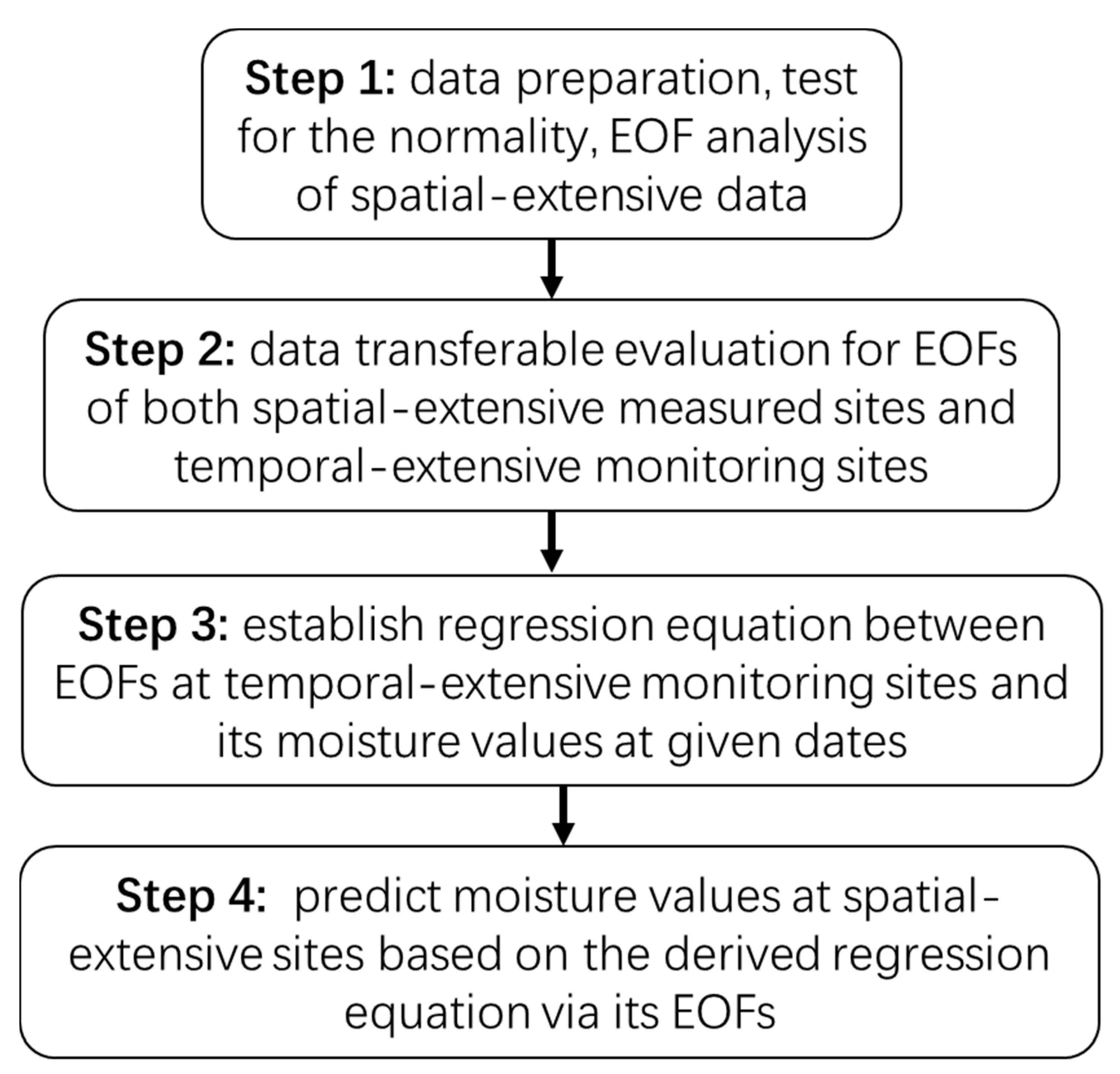
Furthermore, given that the first EOF exhibited the general patterns of soil moisture across the whole investigated spatial coverage, if the EOFs of the manual measurements at some sites had strong correlations with automatically recorded values, then it was possible to apply this relationship to the first EOF to derive the soil moisture across the entire area at any automated monitoring time. Consequently, we considered that this method might have provided an appropriate way to integrate the spatially-extensive (but temporally-limited) manual datasets and the temporally-extensive (but spatially-limited) automated monitoring datasets. The following narrative describes the four steps involved in the data merging methods (Figure 4).
First, an EOF decomposition was performed on the soil moisture dataset to identify the patterns of covariation (the EOFs) and their importance on each date (the ECs).
Second, statistical tests were used to determine the significance of correlation between the EOFs of spatial-extensive measured sites and of temporal-extensive monitoring sites and these should be retained in the transferring method. It is suggested that the EOFs of both datasets are similar in statistical values and regulated with similar contributing factors.
Third, a regression analysis (e.g., multiple linear regression) was performed to identify empirical relationships between automated monitored soil moisture data and its EOFs.
Fourth, the identified empirical relationships were employed to calculate soil moisture at each manual measured site within the entire catchment via its EOFs.
3. Results and Discussion
3.1. Spatial-Temporal Patterns of Soil Moisture
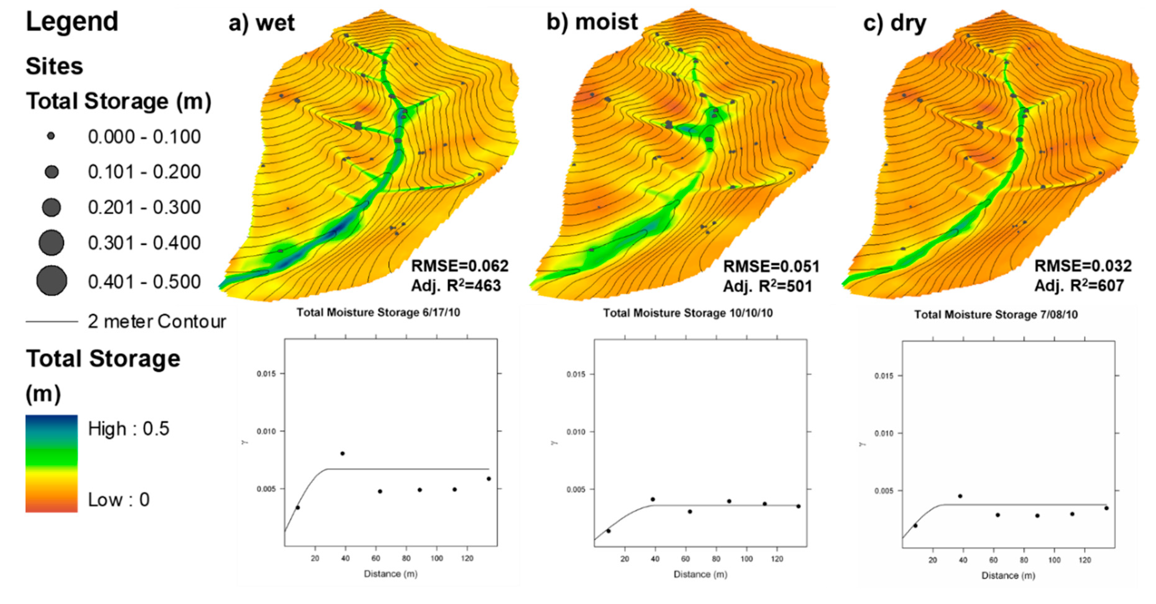
The variogram analysis and the histogram of soil moisture storage indicated that interpolated soil moisture maps exhibited seasonal alignments of soil moisture storage with convergent topographic areas (Figure 5). We found sample variograms with a clear sill and nugget and observed that the geostatistical structure of soil moisture was seasonally evolved. During the wet period, high sills (0.007 m2) and low correlation lengths (20–30 m) were observed, whereas during the dry summer periods, sills were smaller (0.004 m2) and correlation lengths were longer (30–40 m). Relatively low root mean squared error (RMSE) and high coefficient of determination (R2) indicated that regression kriging predicted soil moisture at unmeasured locations with weak kriging error. The RMSE between predicted and observed values generally decreased with decreasing soil wetness, suggesting that regression kriging performed better under dry conditions or at low topographic wetness index (Figure 5). The RMSE also generally increased with soil depth, indicating that the regression kriging with terrain attributes performed better at low values of depth to bedrock [6]. Regardless of the wetness conditions, the swales and the valley floor (i.e., near-stream zone) always showed the wettest conditions. These wet-up and dry-down patterns were consistent with the overall distribution of the soil types and the topographic parameters within the catchment. There was an exponential increase in catchment-wide soil moisture variability with increased averaged-catchment moisture contents [28]. These conditions were evident due to the well-drained and steep-sloped soils within the catchment that confined saturated areas to the swales and the valley floor.
The soil moisture variability was explained using only the first few EOF patterns within the Shale Hills (Table 1). At 10 cm soil depths, the first four EOFs explained approximately 87% of the total variability. In contrast, only the first EOF (or EOF1) explained about 76% of the total soil moisture variance, indicating that a single spatial structure may explain much of the overall soil moisture pattern. With increased soil depths, the total variation presented by the derived EOFs also increased. These results indicated that the seemingly intricate patterns of soil moisture within the investigated catchment might largely be explained by a minimal number of underlying spatial EOFs. In the EOF analysis of spatial patterns, the impact of temporally variable factors, which do not affect the whole area uniformly, also resulted in noise and would be expected to have decreased the amount of the variance explained by the significant EOFs.
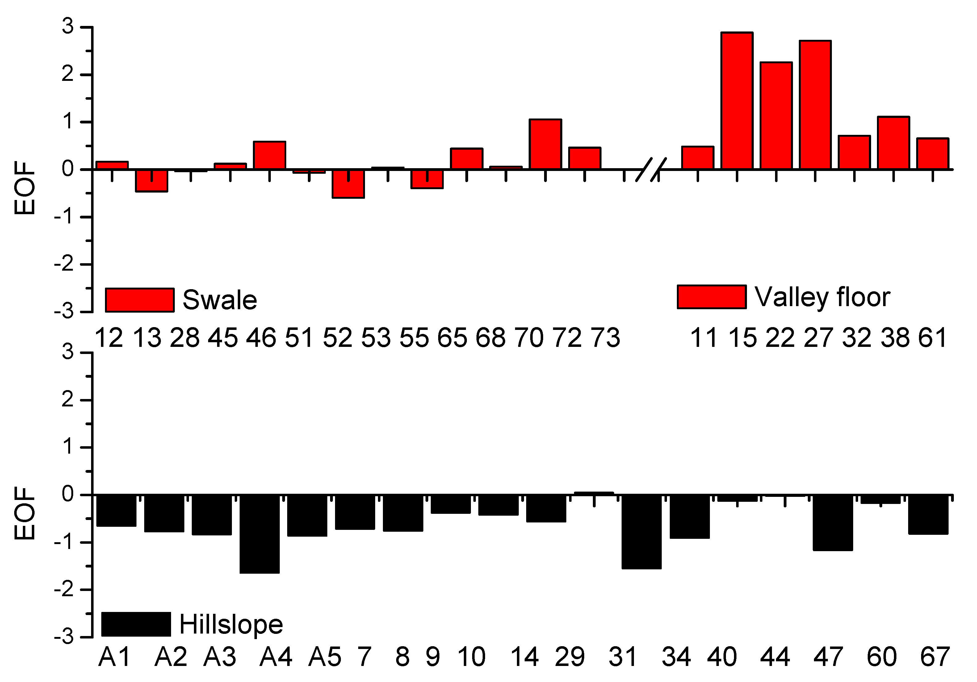
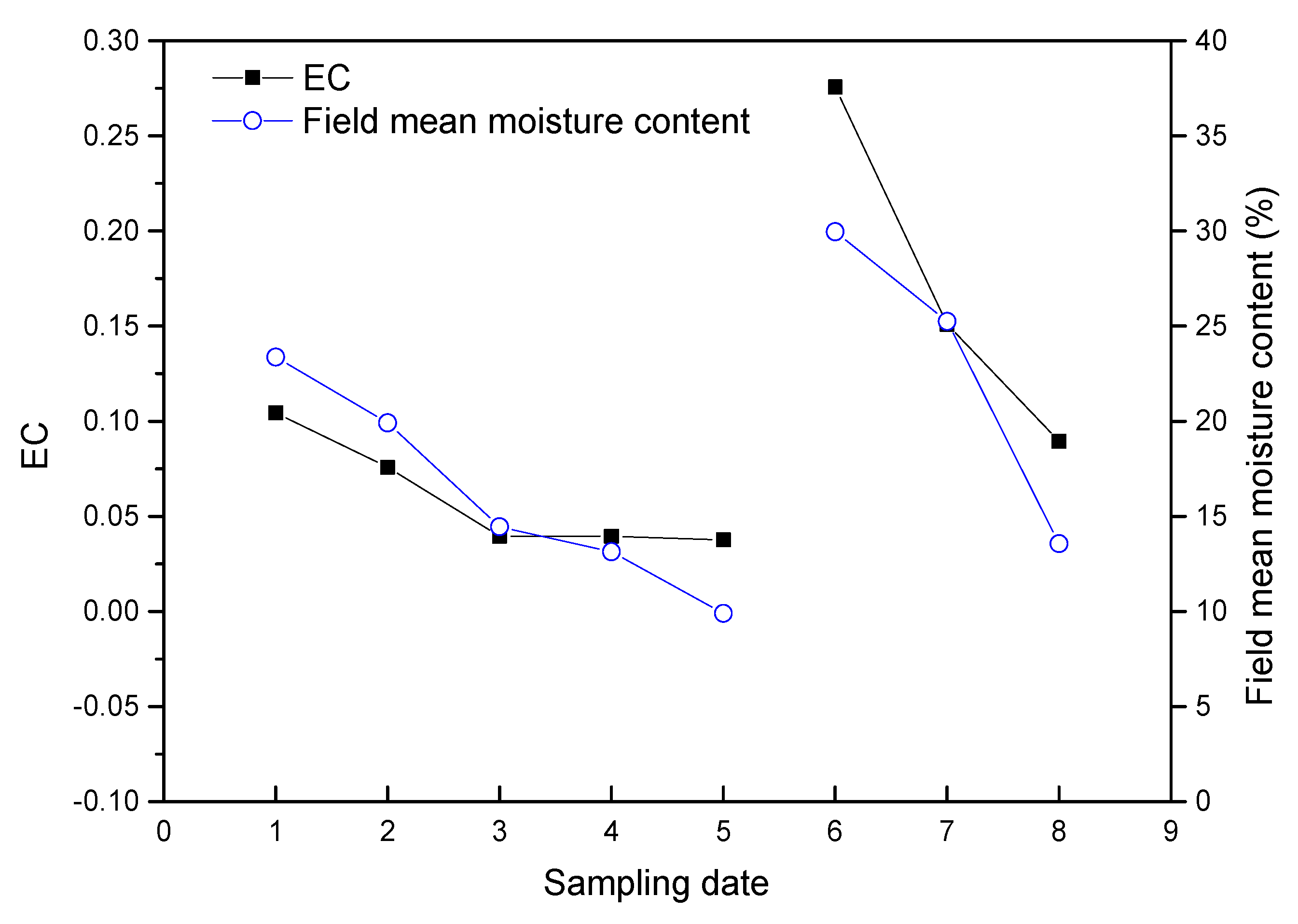
A close examination of the EOF patterns associated with soil land units in Figure 6 reveals that EOF1 displayed high values within the valley floor and low values within the hillslopes, respectively. The high EOF values indicated a clustered site with above-average soil moisture. Conversely, low EOF values are equivalent to the areas of below-average soil moisture values (Figure 6). From the weighted EC series (Figure 7), the variance explained by the EOF1 values closely followed the increased field mean moisture contents, i.e., the variance is sharply increased with increased moisture contents following rainfall recharge. Therefore, the EOF analyses seem to represent a compelling set of tools that help explain the patterns in variance associated with general spatial patterns, the indications of positional characteristics, and temporal dynamics. Perry and Niemann [36] found that the first EOF in their study explained 55% of the soil moisture spatial variability at a 10.5-ha Tarrawarra grassland catchment. The explained variances found at the Shale Hills are higher than the previously mentioned studies, about 55% to 70% of surface soil moisture variability, due to the relatively stable spatial patterns at the study sites [22,36]. Topography exerts a significant influence on soil properties since it affects water and sediment redistribution, soil water and heat budgets, and vegetation distribution [20]. Because of these strong combined soil-topographic effects, the observed soil moisture patterns in the Shale Hills was high and can largely be explained by just a few underlying spatial structures or EOF patterns that are dominantly controlled by the soil parameters and topography.
3.2. Controls of Primary Soil Moisture Patterns
The spatial patterns of soil moisture show the higher Pearson correlation coefficients with soil-topography properties at each measurement depth (Table 1). The results generally indicated that terrain features were larger contributors to the variance in soil moisture than the soil properties. While most of the topographical attributes (e.g., topography wetness index and slope) had strong correlations with the derived EOFs, only soil texture among the soil features showed significant correlations. Soil organic matter displayed lower correlations at the surface soil (0–20 cm). Depth to bedrock, which is related to both soil thickness and topography [37], seems to have had a considerable influence on soil moisture variability at all depths. This result may be confirmed by examining the soil moisture values within the wet locations characterized by the soils with >1 m depth to bedrock. While elevation, slope, and curvature were negatively correlated to soil moisture contents, topographic wetness index and soil silt and clay contents indicated a positive correlation. This result is likely because most soils with deep soil profiles are generally limited to lower elevations and concave slope areas (i.e., valley floor and swales) where soil moisture is usually the highest. Henninger et al. [38] reported that soil moisture increased in the near-stream zone within a predominantly agricultural watershed due to topographic convergence and moderately to poorly drained soils. Our regression analysis indicated that soil texture did not exert a strong influence on the soil moisture spatial distributions at the catchment, probably due to the relatively small variations in soil textural properties throughout the measured locations for the different soil-landform units [34]. Famiglietti [1] reported that, under wet conditions, the best correlations for soil moisture existed with porosity and hydraulic conductivity along with a profile of a 200-m length. In contrast, under dry conditions, soil moisture was well correlated with the relative elevation, aspect, and clay content.
The EOF analysis was repeated for the spatial anomaly data in two categories (depth/wetness), and the degree to which these factors affected the soil moisture distribution was calculated (Table 1). At the Shale Hills, the correlation coefficient values generally increased with soil depth for elevation, slope, and soil silt and clay contents. In contrast, the highest values were observed at intermediate depths (0.4 m) for curvature, depth to bedrock, and topographic wetness index. These results indicate that soil moisture becomes strongly aligned with convergent topography and suggests that lateral flow processes may be an essential driver of soil moisture redistribution at these depths. The increased influence of these parameters with depth may relate to the seasonal changes of soil moisture, which undergoes more dramatic changes near the soil surface. As indicated in Takagi and Lin [6], the subsurface soil moisture exhibited weak temporal variability in the correlation coefficient values that suggest the dampened effects of climate and hydrological fluxes. Thus, the subsurface soil moisture distribution in this catchment is a function of both topographic parameters and soil depth, an observation that was reinforced by the transient hydrological fluxes such as the presence of the temporary shallow water table that seasonally exist within the valley.
3.3. Data Combining Method of Spatially- and Temporally-Extensive Soil Moisture
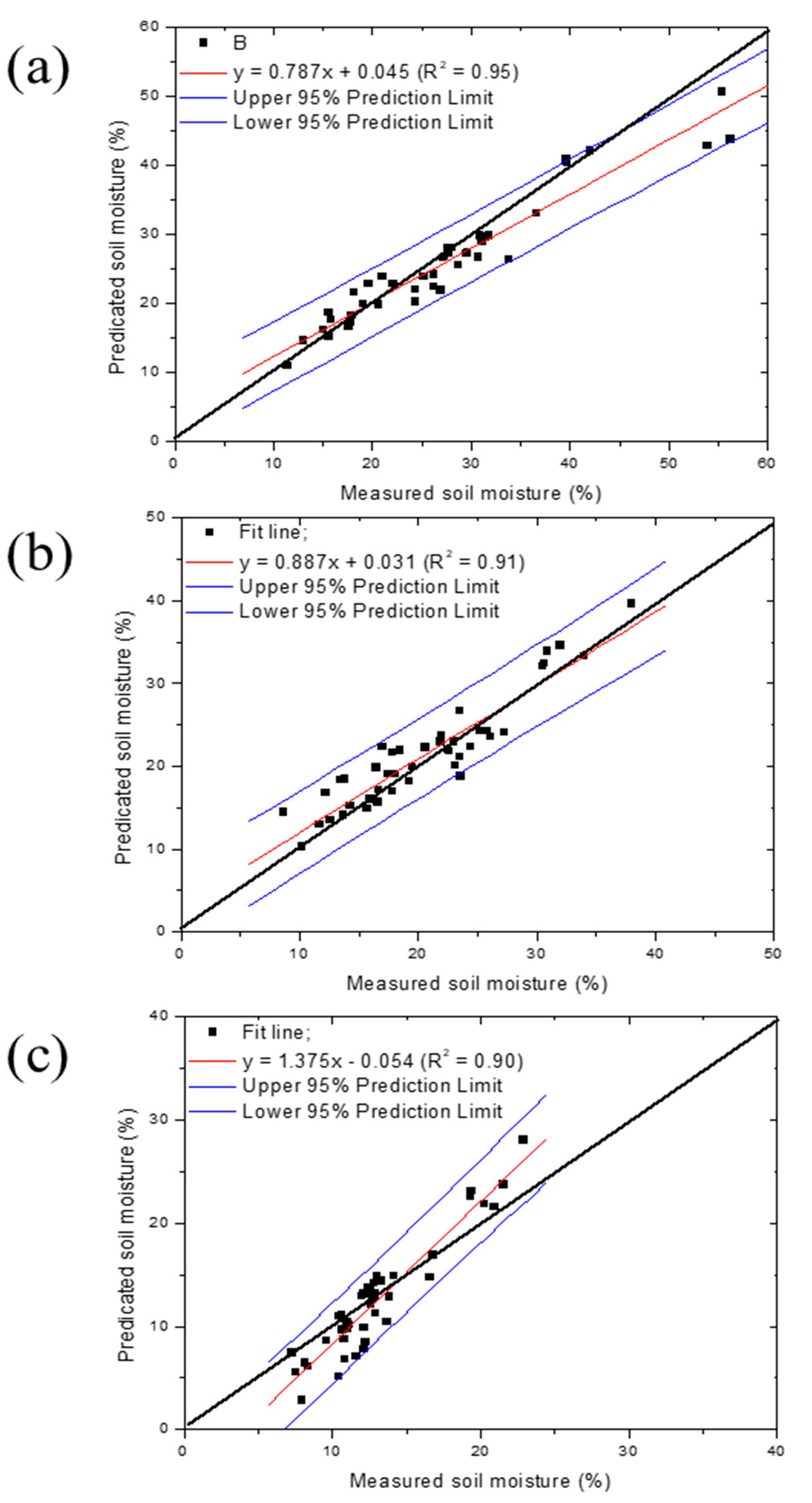
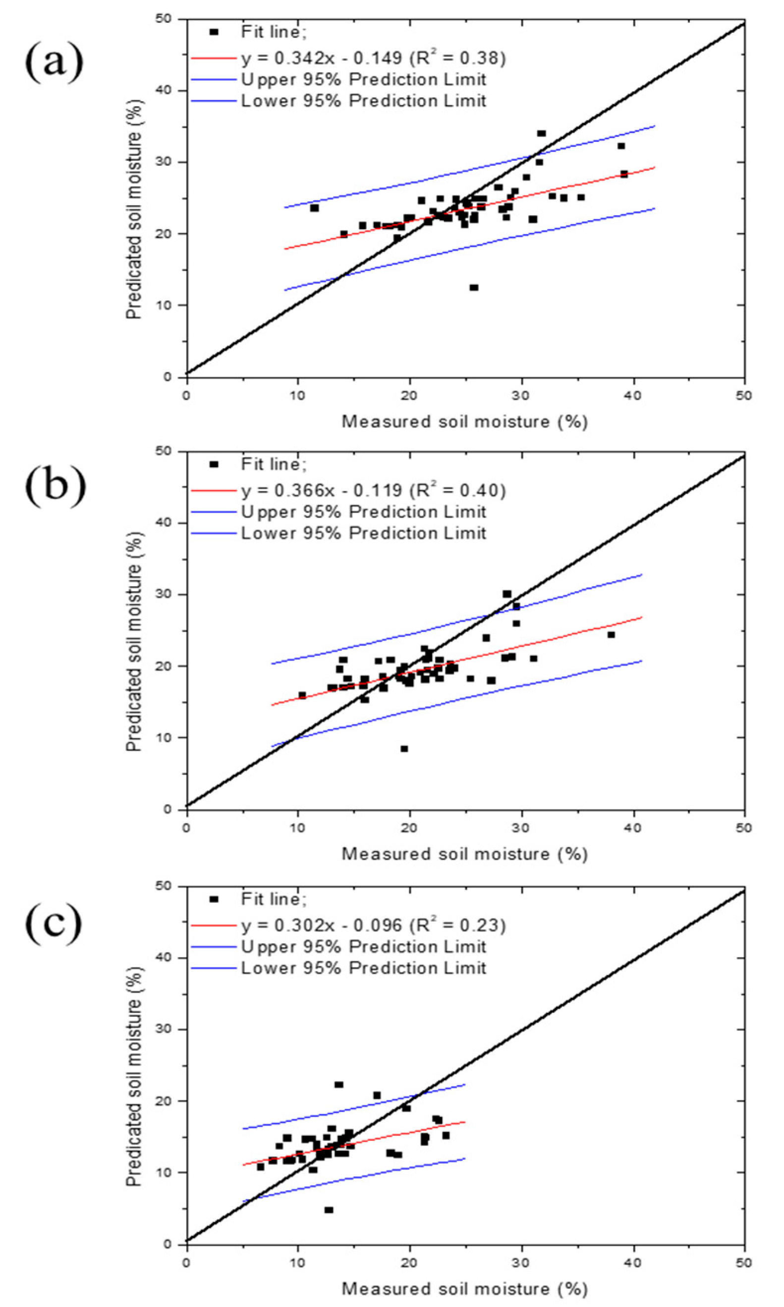
In this study, we found that the first EOF can predict the general patterns of soil moisture, for example, at the 20-cm soil depth, with 85% of the variance explained. Although the relative importance of the first EOF on daily patterns of soil moisture waxes and wanes during soil wetting and drying dynamics, the spatial pattern of the EOF is invariant in time. Therefore, we considered it is an efficient way to integrate the spatially extensive (but temporally limited) manual measurement sites with other fields of long-term monitoring datasets that are temporally extensive (but spatially limited). Conceivably, based on the EOFs for all spatially extensive sites, it is possible to predict the spatially-distributed soil moisture for all those sites, based on the derived regressive equation between the EOFs of the temporally-extensive sites and the automated monitoring datasets. For instance, the first EOF of soil moisture at 20-cm soil depth was derived from a manual dataset with higher explained variations. Still, there was a strong-correlated regression coefficient between the soil moisture automated monitoring sites (e.g., five sites 15, 51, 55, 61, and 74) and their corresponding EOF values. Based on the derived equations, all manual measurement values could be predicted by either the manual measurements or the monitored values at those five monitoring sites. To validate this assumption, we selected three wetness conditions on the same dates as used in Figure 5 (i.e., wet: 6 May 2010; moist: 17 June 2010; dry: 8 July 2010). Remarkably, the predicted values via the manually-measured data (Figure 8) have a strong linear correlation to the measurements, with high confidence levels (95%). These results mean that the suggested method is a practical means to combine the manually-measured datasets with the automatically-monitored datasets. This facilitated the analysis of soil moisture response dynamics, and thus made it possible to better identify several patterns which can be attributed to different phenomena of the unsaturated water flow [32,39].
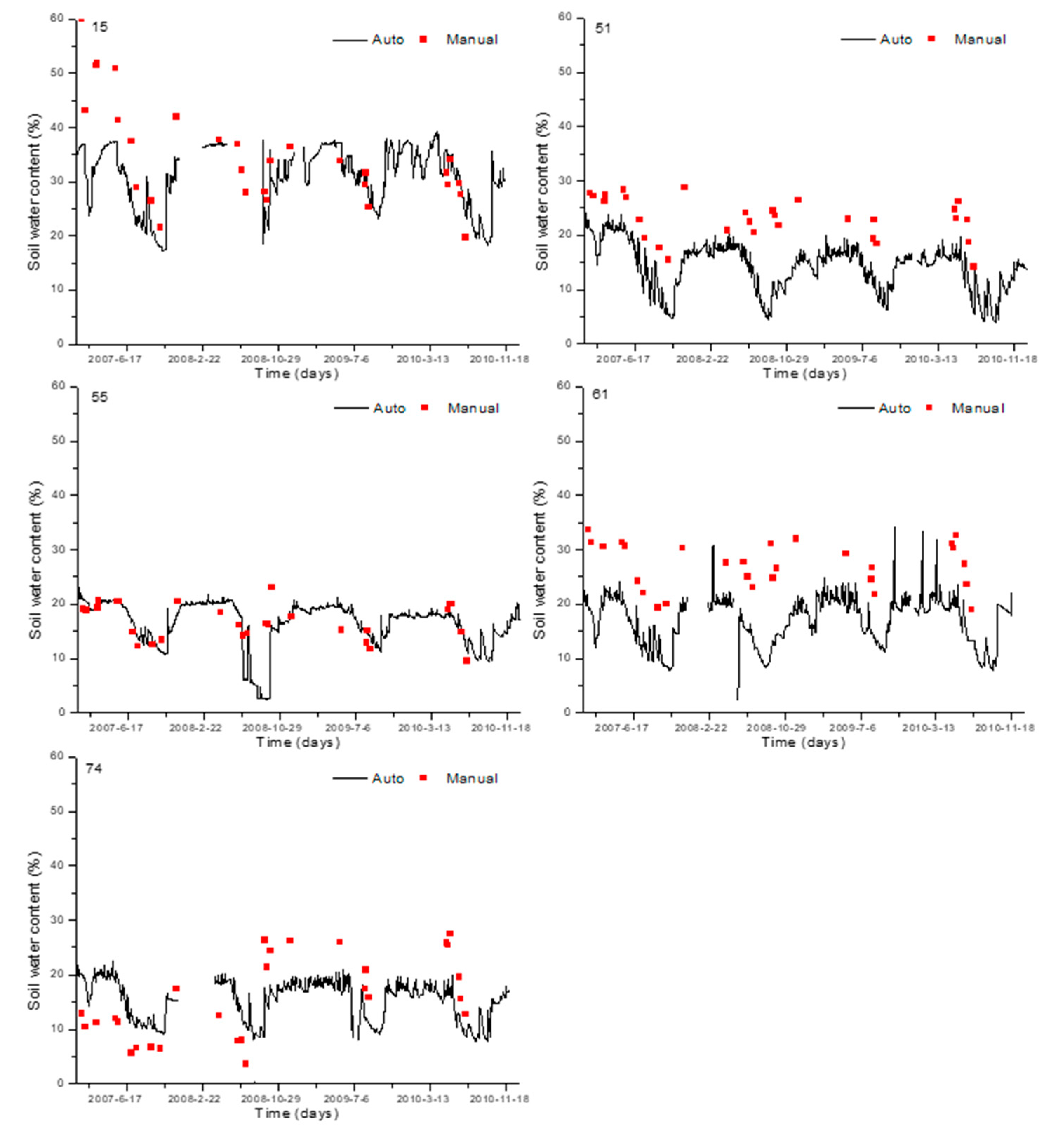
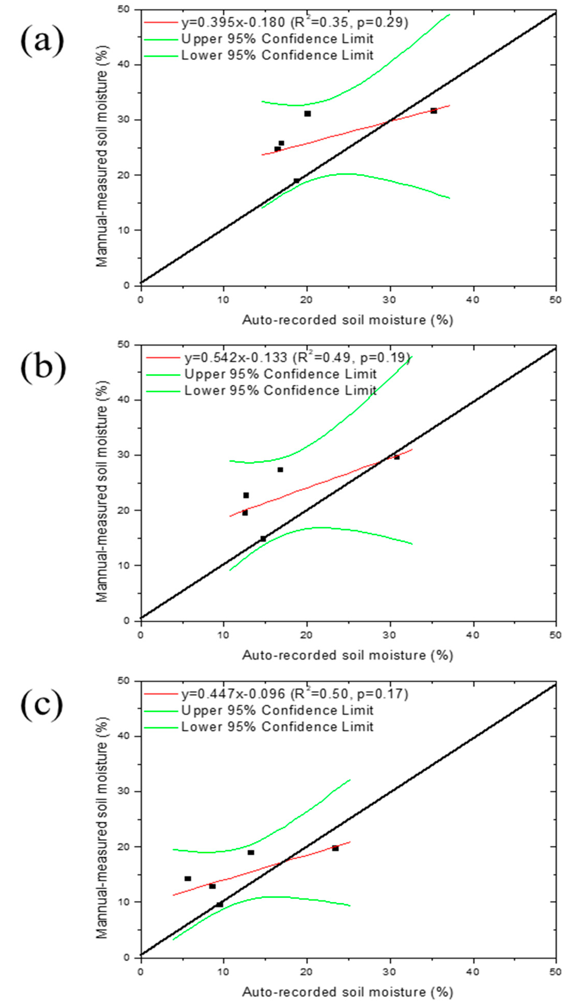
Note that the results showed a relatively large scatter when the automatically-monitored values were used to predicate soil moisture values at the spatially extensive sites (Figure 9). Whether this approach is accurate is also dependent on how well the manually-measured data and the automatically-monitored data closely match for the same soil depths at the same sites. Due to the differences in the measured thickness and horizonation, spatial dimensions, and scales for the two methods [40], the values of manually-measured and automated-monitored datasets may not necessarily match well. As indicated in Figure 10, except for site 55, there were large differences between manually-measured and automatically-monitored soil moisture values. For instance, the manually-measured moisture contents were consistently higher than the automatically-monitored values for site 51 during the entire measurement period. Even worse, the trends between both datasets for sites 15 and 74 are somewhat irregular. These results challenged the suitability of using the automated-monitored data, instead of the manually-measured data, at the temporally-limited site. As shown in Figure 11, we found that the fit between manual-measured and auto-recorded soil moisture datasets were significant but relatively weak. Therefore, to apply this method reasonably, it is essential for predicted data accuracy accounting that the manually-measured and automatically-monitored data be somewhat in agreement. It is expected that the EOF method could be a practical and efficient data merging method if the primary EOF explains >60% of the variation, and therefore data transferability is guaranteed. Nevertheless, taking into account those differences, the EOF method, as applied in this study, could be quite valuable, and therefore provide an essential way to assimilate data from multiple sources.
Furthermore, we explored the EOF method to breakdown a more dynamic time series of soil moisture into a lesser number of orthogonal spatial EOF patterns (that are invariant in time) and corresponding EC components (that are invariant in space). This modification dramatically simplifies our task as we can just deal with only a few spatial EOF structures instead of the whole data set (Table 1). The higher-order EOFs are usually taken into account, depending on the total variance explained by them. The associated EC components show the variation in the influence of the EOFs during the wetting/drying phases, which could be reasonably associated with the automated monitoring moisture dynamics and theoretically provide the basis for the data fusion. To determine the dominant physical controls of soil moisture, the EOF patterns were tested for correlation with the soil-terrain characteristics of the region. From our analyses, we inferred that variabilities in the soil moisture EOF patterns are related to both topography and soil texture. We assessed that the EOF analysis is particularly applicable to combine the manual datasets with the monitoring datasets in terms of different resolutions for different data sources. The soil moisture dataset currently provides either better spatial coverage or better temporal coverage, thus producing either spatial soil moisture patterns or information on the dynamics [28]. In this regard, our data assimilation approach has demonstrated an opportunistic and holistic combination of two pre-existing data sources. As a result, this approach offers a meaningful way to combine both datasets, which certainly improved the explanations for the variation and data use. Besides, at the same catchment, the previous result indicated that the number of annual measurement sites needed to reliably estimate (i.e., with 95% confidence and ±0.05 m3 m−3 tolerance) the catchment-wide mean soil moisture varied between 2 and 38 depending on wetness/depth/season [34]. This means that, for future measurements of the Shale Hills and other similar catchments, the spatial sampling locations could be reduced to a much lower number.
3.4. Implications
Existing methods for direct field measurement of soil moisture remain time-consuming and costly. Significant spatial and temporal variability challenges the possibility of understanding the underlying hydrological process and mechanisms [13,20]. However, the spatial pattern, as indicated by the EOF analysis, is relatively stable. This stability attribute implies that it is possible to assess the soil moisture distribution in a catchment continuously. In addition to the spatial coverage maps, adding the long-term monitoring of surface and subsurface soil moisture provides a comprehensive picture of the spatial-temporal pattern of soil moisture dynamics across the whole area. This allows the identification of factors that influence it through time. A unique long-term real-time soil moisture data set was previously used to identify local dominant hydrological processes and their temporal dynamics. In this perspective, our approach becomes more significant, given that the long-term monitored site is characterized as a time-stable location via a time-stability analysis [41]. Our practice can also assimilate additional data sources, e.g., remotely sensed data at this time-stable site. Given the high accuracy of the soil moisture monitoring, the high temporal resolution soil moisture patterns over an area could be obtained by selecting a temporally stable monitoring site, which is useful in ground-truthing of a remotely sensed footprint for validation of simulation modeling results, and also in the extension of soil moisture at depth, given remote sensing estimates limited to the top few centimeters of the soil [34,41]. Given the importance of soil moisture in the Earth’s land surface interactions and its vast potential applications, accurate estimation is vital in addressing some practical challenges such as food security, sustainable soil management, and water resource maintenance. The new approach of remote sensing strengthens innovative research and scientific inventions that will lead to advancements [20].
One goal of this study was to lay the foundation for the design of efficient real-time soil moisture monitoring networks that fill the gap between point sensors and traditional manual measurements, or even remote sensing values. Our study represents a novel approach with potential benefits for an effective soil moisture monitoring network design within the study area, determining the spatiotemporal statistics of the observed soil moisture fields, and using a spatial regression procedure in data merging. It is more realistic to observe a difference between developed maps as surface conditions evolve. Obviously, the combination of data sets with different spatiotemporal resolution have synergetic effects and thus yield additional insights [32]. The findings of this study have demonstrated the ability of a limited number of monitoring sites to provide accurate estimates of large-scale soil moisture patterns [33]. This combination reflects the field heterogeneity and complex interactions between soil moisture and its controlling factors, which will help the investigation of subsurface water flow processes. Although there are simple linear data transfer methods can be applied to this type, our approach may accommodate different data analysis methods, such as a multi-step regression method based on EOF analysis, using ancillary information and hybrid methods [42]. It could also be interesting to have more strict validation against independent data, such as the K-fold cross validation. Once we have completed such tasks, the EOF-based transfer method may be used as a foundation for any region and date, given that the identified empirical relationships will be valid for the application conditions.
The practical effectiveness of our data merging approach might have implied that the catchment was well shaped by a combination of long- and short-time processes and this information has been assumed to provide some clues in order to project future changes. It is challenging to link such long-term and slow processes with shorter-term and fast processes [13]. While mapping depicts the spatial distribution of soil-landscape relationships, as indicated by the dominant EOF patterns, monitoring captures the temporal dynamics of hydrologic properties and climate information, as noted in the profiled data dynamics. Given the spatial-extensive data benefits of traditional mapping and the temporal-extensive data benefits of conventional monitoring, the presented data-integrated method may provide a justifiable basis for the combination of mapped and monitored data, as well as a conceptual basis for the coupling of slow and fast processes. Firstly, bridging mapping with monitoring is undoubtedly helpful in the dynamic mapping of hydro-pedologic functional units [13]. Secondly, mapping supplies information to aid in optimal site selection for monitoring, particularly in identifying the time-stable point to assist in the scaling and modeling of the landscape–soil–water dynamics [41]. Thirdly, mapping and monitoring identifies the dominant control of soil moisture in modeling hydrological processes, delivers essential data for modeling calibration and validation, and may help provide additional information for more proper management of soil and water resources [43]. Our approach has established an essential set of tools to evaluate the improvement of data use and proved to be less expensive than the high-density installation of continuously logging sensors while also applying to a complicated catchment. This extensive data set provides a unique opportunity to improve our understanding of other catchment-scale processes, particularly under projected climate change. We have assumed that the relationship between different data sources remains the same over time but suggest that future studies verify this behavior.
4. Conclusions
In this study, we developed a data combination approach based on EOF analysis of space-time soil moisture data at a reference Shale Hills catchment. We investigated the space-time characterization of soil moisture and found that the variation of soil moisture could be explained by using the first few EOFs. Results of the correlation analysis showed that topography and soil properties have mixed effects on the variability explained by the dominant soil moisture EOFs. Benefits based on the derived underlying stable EOF patterns of soil moisture, the relationships between site characteristics, and EOF patterns were examined to conduct a spatial-temporal dataset combination. Based on the long-term spatial extensive sampling campaign and the specific transect of real-time monitoring, this study investigated how to integrate spatially extensive, but temporally limited manual datasets with temporally extensive, but spatially limited automated monitoring datasets. This exercise has contributed to understanding soil moisture spatio-temporal patterns and hydrological responses at a small landscape scale, considered to be essential tools for the useful measurement and the practical management of soil moisture at multiple scales.
Author Contributions
Y.Z. analyzed the data; Y.Z., F.L. and R.Y. contributed reagents/materials/analysis tools; Y.Z. wrote the manuscript. F.L., W.J., and R.L.H. reviewed and edited the manuscript. All authors have read and agree to the published version of the manuscript.
Funding
This research was supported in part by the U.S. National Science Foundation through the Shale Hills Critical Zone Observatory grant (EAR-0725019), the Taishan Scholars Program (201812096), and the National Natural Science Foundation of China (41977009). Fei Li was supported by the Agricultural Science and Technology Innovation Program of CAAS (CAAS-ASTIP-2020-IGR-04). Hill was partially supported by the USDA National Institute of Food and Agriculture, Hatch project 1014496.
Acknowledgments
Assistance in field data collections from the Penn State Hydropedology Group was gratefully acknowledged.
Conflicts of Interest
The authors declare no conflict of interest.
References
- Famiglietti, J.S.; Rudnicki, J.W.; Rodell, M. Variability in surface moisture content along a hillslope transect: Rattlesnake Hill, Texas. J. Hydrol. 1998, 210, 259–281. [Google Scholar] [CrossRef] [Green Version]
- Korres, W.; Reichenau, T.G.; Fiener, P.; Koyama, C.N.; Bogena, H.R.; Cornelissen, T.; Baatz, R.; Herbst, M.; Diekkrüger, B.; Vereecken, H.; et al. Spatio-temporal soil moisture patterns-A meta-analysis using plot to catchment scale. J. Hydrol. 2015, 520, 326–341. [Google Scholar] [CrossRef] [Green Version]
- Grayson, R.B.; Blöschl, G.; Western, A.W.; McMahon, T.A. Advances in the use of observed spatial patterns of catchment hydrological response. Adv. Water Resour. 2002, 25, 1313–1334. [Google Scholar] [CrossRef]
- Lin, H.S. Temporal stability of soil moisture spatial pattern and subsurface preferential flow pathways in the Shale Hills Catchment. Vadose Zone J. 2006, 5, 317–340. [Google Scholar] [CrossRef]
- Famiglietti, J.S.; Ryu, D.; Berg, A.A.; Rodell, M.; Jackson, T.J. Field observations of soil moisture variability across scales. Water Resour. Res. 2008, 44, W01423. [Google Scholar] [CrossRef] [Green Version]
- Takagi, K.; Lin, H.S. Changing controls of soil moisture spatial organization in the Shale Hills Catchment. Geoderma 2012, 173–174, 289–302. [Google Scholar] [CrossRef]
- Owe, M.; Jones, E.B.; Schmugge, T.J. Soil moisture variation patterns observed in Hand Country, South Dakota. Water Resour. Bull. 1982, 18, 949–954. [Google Scholar] [CrossRef] [Green Version]
- Grayson, R.B.; Western, A.W.; Chiew, F.H.S.; Blöschl, G. Preferred states in spatial soil moisture patterns: Local and non local controls. Water Resour. Res. 1997, 33, 2897–2908. [Google Scholar] [CrossRef]
- Zhu, Q.; Lin, H.S. Interpolation of soil properties based on combined information of spatial structure, sample size and auxiliary variables. Pedosphere 2010, 20, 594–606. [Google Scholar] [CrossRef]
- Shi, Y.; Baldwin, D.C.; Davis, K.J.; Yu, X.; Duffy, C.J.; Lin, H. Simulating high-resolution soil moisture patterns in the Shale Hills watershed using a land surface hydrologic model. Hydrol. Process. 2015, 29, 4624–4637. [Google Scholar] [CrossRef]
- Dunn, S.M.; Lilly, A. Investigating the relationship between a soils classification and the spatial parameters of a conceptual catchment-scale hydrological model. J. Hydrol. 2001, 252, 157–173. [Google Scholar] [CrossRef]
- Joshi, C.B.; Mohanty, B.P. Physical controls of near surface soil moisture across varying spatial scales in an agricultural landscape during SMEX02. Water Resour. Res. 2010, 46, W12503. [Google Scholar] [CrossRef] [Green Version]
- Ma, Y.; Li, X.; Guo, L.; Lin, H. Hydropedology: Interactions between pedologic and hydrologic processes across spatiotemporal scales. Earth Sci. Rev. 2017, 171, 181–195. [Google Scholar] [CrossRef]
- Beven, K.; Asadullah, A.; Bates, P.; Blyth, E.; Chappell, N.; Child, S.; Cloke, H.; Dadson, S.; Everard, N.; Fowler, H.J.; et al. Developing observational methods to drive future hydrological science: Can we make a start as a community? Hydrol. Proc. 2020, 34, 868–873. [Google Scholar] [CrossRef] [Green Version]
- Western, A.W.; Grayson, R.B.; Blöschl, G.; Willgoose, G.R.; McMahon, T.A. Observed spatial organization of soil moisture and its relation to terrain indices. Water Resour. Res. 1999, 35, 797–810. [Google Scholar] [CrossRef] [Green Version]
- Baldwin, D.; Naithani, K.J.; Lin, H. Combined soil-terrain stratification for characterizing catchment-scale soil moisture variation. Geoderma 2017, 285, 260–269. [Google Scholar] [CrossRef] [Green Version]
- Lin, H.S.; Bouma, J.; Pachepsky, Y.; Western, A.W.; Thompson, J.A.; van Genuchten, M.T.; Vogel, H.; Lilly, A. Hydropedology: Synergistic integration of pedology and hydrology. Water Resour. Res. 2006, 42, W05301. [Google Scholar] [CrossRef]
- Buttafuoco, G.; Castrignanò, A.; Cucci, G.; Lacolla, G.; Lucà, F. Geostatistical modelling of within-field soil and yield variability for management zones delineation: A case study in a durum wheat field. Precis. Agric. 2017, 18, 37–58. [Google Scholar] [CrossRef]
- Western, A.W.; Grayson, R.B.; Blöschl, G. Scaling of soil moisture: A hydrologic perspective. Ann. Rev. Earth Planet. Sci. 2002, 30, 149–180. [Google Scholar] [CrossRef] [Green Version]
- Lucà, F.; Buttafuoco, G.; Terranova, O. GIS and soil. In Comprehensive Geographic Information Systems; Huang, B., Ed.; Elsevier: Oxford, UK, 2018; Volume 2, pp. 37–50. [Google Scholar]
- D’Odorico, P.; Porporato, A. Preferential states in soil moisture and climate dynamics. Proc. Natl. Acad. Sci. USA 2004, 101, 8848–8851. [Google Scholar] [CrossRef] [Green Version]
- James, A.L.; Roulet, N.T. Antecedent moisture conditions and catchment morphology as controls on spatial patterns of runoff generation in small forest catchments. J. Hydrol. 2009, 377, 351–366. [Google Scholar] [CrossRef]
- Deiana, R.; Cassiani, G.; Villa, A.; Bagliani, A.; Bruno, V. Calibration of a vadose zone model using water injection monitored by GPR and electrical resistant tomography. Vadose Zone J. 2008, 7, 215–226. [Google Scholar] [CrossRef]
- Guo, L.; Lin, H.; Fan, B.; Nyquist, J.; Toran, L.; Mount, G. Preferential flow through shallow fractured bedrock and a 3D fill-and-spill model of hillslope subsurface hydrology. J. Hydrol. 2019, 576, 430–442. [Google Scholar] [CrossRef]
- Ben-Dor, E. Quantitative remote sensing of soil properties. Adv. Agron. 2002, 75, 173–243. [Google Scholar]
- Zhao, Y.; Peth, S.; Horn, R.; Hallett, P.; Wang, X.Y.; Giese, M.; Gao, Y.Z. Factors controlling the spatial patterns of soil moisture investigated by multivariate and geostatistical analysis. Ecohydrology 2011, 4, 36–48. [Google Scholar] [CrossRef]
- Jawson, S.D.; Niemann, J.D. Spatial patterns from EOF analysis of soil moisture at a large scale and their dependence on soil, landuse, and topographic properties. Adv. Water Resour. 2007, 30, 366–381. [Google Scholar] [CrossRef]
- Zhao, Y.; Tang, J.; Zhu, Q.; Takagi, K.; Graham, C.B.; Lin, H. Hydropedology in the ridge and valley: Soil moisture patterns and preferential flow dynamics in two contrasting landscapes. In Hydropedology (Chapter 12); Lin, H., Ed.; Academic Press: Cambridge, MA, USA, 2012; pp. 381–411. [Google Scholar]
- Yoo, C.; Kim, S. EOF analysis of surface soil moisture field variability. Adv. Water Resour. 2004, 27, 831–842. [Google Scholar] [CrossRef]
- Wagenet, R.J. Scale issues in agroecological research chains. Nutr. Cycl. Agroecosyst. 1998, 50, 23–34. [Google Scholar] [CrossRef]
- Martini, E.; Wollschläger, U.; Musolff, A.; Werban, U.; Zacharias, S. Principal component analysis of the spatiotemporal pattern of soil moisture and apparent electrical conductivity. Vadose Zone J. 2017, 16, 1–12. [Google Scholar] [CrossRef]
- Blume, T.; Zehe, E.; Bronstert, A. Use of soil moisture dynamics and patterns at different spatio-temporal scales for the investigation of subsurface flow processes. Hydrol. Earth Syst. Sci. 2009, 13, 1215–1234. [Google Scholar] [CrossRef] [Green Version]
- Martinez, C.; Hancock, G.R.; Kalma, J.D.; Wells, T. Spatiotemporal distribution of near-surface and root zone soil moisture at the catchment scale. Hydrol. Process. 2008, 22, 2699–2714. [Google Scholar] [CrossRef]
- Takagi, K.; Lin, H.S. Temporal dynamics of soil moisture spatial variability in the shale hills critical zone observatory. Vadose Zone J. 2011, 10, 832–842. [Google Scholar] [CrossRef]
- Lin, H.; Zhou, X. Evidence of subsurface preferential flow using soil hydrologic monitoring in the Shale Hills catchment. Eur. J. Soil Sci. 2008, 59, 34–49. [Google Scholar] [CrossRef]
- Perry, M.A.; Niemann, J.D. Generation of soil moisture patterns at the catchment scale by EOF interpolation. Hydrol. Earth. Syst. Sci. 2008, 12, 39–53. [Google Scholar] [CrossRef] [Green Version]
- Lucà, F.; Buttafuoco, G.; Robustelli, G.; Malafronte, A. Spatial modelling and uncertainty assessment of pyroclastic cover thickness in the Sorrento Peninsula. Environ. Earth Sci. 2014, 72, 3353–3367. [Google Scholar] [CrossRef]
- Henninger, D.L.; Peterson, G.W.; Engman, E.T. Surface soil moisture within a watershed: Variations, factors influencing, and relationships to surface runoff. Soil Sci. Soc. Am. J. 1976, 40, 773–776. [Google Scholar] [CrossRef]
- Brocca, L.; Morbidelli, R.; Melone, F.; Moramarco, T. Soil moisture spatial variability in experimental areas of central Italy. J. Hydrol. 2007, 333, 356–373. [Google Scholar] [CrossRef]
- Gu, W.Z.; Liu, J.F.; Lin, H.S.; Lin, J.; Liu, H.W.; Liao, A.-M.; Wang, N.; Wang, W.Z.; Ma, T.; Yang, N.; et al. Why hydrological maze: The hydropedological trigger? Review of experiments at Chuzhou Hydrology Laboratory. Vadose Zone J. 2018, 17, 170174. [Google Scholar] [CrossRef] [Green Version]
- Zhao, Y.; Peth, S.; Wang, X.Y.; Lin, H.S.; Horn, R. Temporal stability of surface soil moisture spatial patterns and their controlling factors in a semi-arid steppe. Hydrol. Proc. 2010, 24, 2507–2519. [Google Scholar] [CrossRef]
- Temimi, M.; Leconte, R.; Chaouch, N.; Sukumal, P.; Khanbilvardi, R.; Brissette, F. A combination of remote sensing data and topographic attributes for the spatial and temporal monitoring of soil wetness. J. Hydrol. 2010, 388, 28–40. [Google Scholar] [CrossRef]
- Koster, R.D.; Dirmeyer, P.A.; Guo, Z.; Bonan, G.; Chan, E.; Cox, P.; Gordon, C.T.; Kanae, S.; Kowalczyk, E.; Lawrence, D.; et al. Regions of strong coupling between soil moisture and precipitation. Science 2004, 305, 1138–1140. [Google Scholar] [CrossRef] [PubMed] [Green Version]
Figure 1.
Map of the Shale Hills catchment and the location of soil moisture measurement sites used in this study. The number in the figure indicates the site location. The shaded polygon is the ridge-swale sub-unit.
Figure 1.
Map of the Shale Hills catchment and the location of soil moisture measurement sites used in this study. The number in the figure indicates the site location. The shaded polygon is the ridge-swale sub-unit.

Figure 2.
Maps of soil and terrain attribute in the Shale Hills catchment. Maps were interpolated using regression kriging. (a) DB: depth to bedrock, (b) Clay: clay content, (c) Silt: silt content, and (d) RF: rock fragment.
Figure 2.
Maps of soil and terrain attribute in the Shale Hills catchment. Maps were interpolated using regression kriging. (a) DB: depth to bedrock, (b) Clay: clay content, (c) Silt: silt content, and (d) RF: rock fragment.

Figure 3.
Maps of topographical attributes in the Shale Hills catchment. Maps were created using smoothed digital elevation model (DEM). (a) E: elevation, (b) TWI: topographic wetness index; (c) SP: slope percent, (d) UCA: upslope contributing area, and (e) PC: profile curvature.
Figure 3.
Maps of topographical attributes in the Shale Hills catchment. Maps were created using smoothed digital elevation model (DEM). (a) E: elevation, (b) TWI: topographic wetness index; (c) SP: slope percent, (d) UCA: upslope contributing area, and (e) PC: profile curvature.

Figure 4.
The flow diagram of the data merging approach based on Empirical Orthogonal Function (EOF) analysis.
Figure 4.
The flow diagram of the data merging approach based on Empirical Orthogonal Function (EOF) analysis.

Figure 5.
Representative maps of soil moisture storage, along with corresponding semi-variograms (γ), under (a) wet, (b) moist, and (c) dry conditions. Maps were interpolated using regression kriging. RMSE: Root mean squared error. Adj. R2 represents the adjusted R2 for regression kriging. Appropriate model functions were fitted to the semi-variogram obtained by the maximum likelihood cross-validation method. Before applying the geostatistical tests, each variable was also checked for drift, trend and anisotropy. Data were modified from Zhao et al. (2012).

Figure 6.
The first EOFs, along with the different soil land units. The x-axis indicates sampling site numbers labeled in Figure 1.
Figure 6.
The first EOFs, along with the different soil land units. The x-axis indicates sampling site numbers labeled in Figure 1.

Figure 7.
Weighted expansion coefficient (EC) time series of EOFs, associated with the field mean moisture content during 2005 (sampling dates from 1–5) and 2007 years (sampling dates from 6–7).
Figure 7.
Weighted expansion coefficient (EC) time series of EOFs, associated with the field mean moisture content during 2005 (sampling dates from 1–5) and 2007 years (sampling dates from 6–7).

Figure 8.
Regression between predicated soil moisture by EOF method using manual datasets and measure datasets exemplified by 20 cm soil depth. For the comparison, we selected three wetness conditions as on the same dates used in Figure 5 under (a) wet, (b) moist, and (c) dry conditions.
Figure 8.
Regression between predicated soil moisture by EOF method using manual datasets and measure datasets exemplified by 20 cm soil depth. For the comparison, we selected three wetness conditions as on the same dates used in Figure 5 under (a) wet, (b) moist, and (c) dry conditions.

Figure 9.
Regression between predicated soil moisture by EOF method using automated datasets and measures datasets exemplified by 20 cm soil depth. For the comparison, we selected three wetness conditions as on the same dates used in Figure 5 under (a) wet, (b) moist, and (c) dry conditions.
Figure 9.
Regression between predicated soil moisture by EOF method using automated datasets and measures datasets exemplified by 20 cm soil depth. For the comparison, we selected three wetness conditions as on the same dates used in Figure 5 under (a) wet, (b) moist, and (c) dry conditions.

Figure 10.
Comparison between auto-monitored and manual-measured soil moisture for 20-cm soil depth at the five long-term monitoring sites (15, 51, 55, 61, and 74).
Figure 10.
Comparison between auto-monitored and manual-measured soil moisture for 20-cm soil depth at the five long-term monitoring sites (15, 51, 55, 61, and 74).

Figure 11.
Regression between manual-measured and auto-recorded soil moisture datasets for 20 cm soil depth at the five long-term monitoring sites. For the comparison, we selected three wetness conditions as on the same dates used in Figure 5 under (a) wet, (b) moist, and (c) dry conditions.
Figure 11.
Regression between manual-measured and auto-recorded soil moisture datasets for 20 cm soil depth at the five long-term monitoring sites. For the comparison, we selected three wetness conditions as on the same dates used in Figure 5 under (a) wet, (b) moist, and (c) dry conditions.


Table 1.
Pearson correlation between Empirical Orthogonal Functions (EOFs) of soil moisture and soil-terrain attributes in the Shale Hill catchment. The numbers in parentheses after each EOF indicate the cumulative total variability explained. DB: depth to bedrock; Clay: clay content; Silt: silt content; and RF: rock fragment; E: elevation; TWI: topographic wetness index; SP: slope percent; UCA: upslope contribution area; PC: profile curvature. Modified from Zhao et al. (2012).
| Depth | EOFs | DB | Clay | Silt | RF | E | TWI | SP | UCA | PC |
|---|---|---|---|---|---|---|---|---|---|---|
| 10 cm | EOF1 (75.5%) | ** | ** | ** | ** | ** | ||||
| EOF2 (79.7%) | ** | ** | ** | ** | ** | ** | ** | ** | ||
| EOF3 (83.5%) | * | |||||||||
| EOF4 (86.8%) | ** | |||||||||
| 20 cm | EOF1 (85.2%) | ** | ** | ** | ** | ** | ** | ** | ** | |
| 40 cm | EOF1 (89.7%) | * | * | * | ** | |||||
| EOF2 (92.7%) | * | ** | ** | ** | ** | |||||
| 60 cm | EOF1 (83.5%) | ** | * | * | * | |||||
| EOF2 (89.2%) | * | * | * | |||||||
| EOF3 (92.1%) | * | * | * | ** | ** | |||||
| 80 cm | EOF1 (87.2%) | ** | ** | ** | * | ** | ** | |||
| EOF2 (91.8%) | ** | ** | * | |||||||
| 100 cm | EOF1 (88.9%) | ** | ||||||||
| EOF2 (92.9%) | ** | ** | * | |||||||
| EOF3 (95.8%) | ||||||||||
| 0–0.1 | 0.1–0.2 | 0.2–0.3 | 0.3–0.4 | 0.4–0.5 | 0.5–0.6 | 0.6–0.7 | 0.7–0.8 | 0.8–0.9 | 0.9–1.0 | |
| Correlation coefficient scale | * significant at p < 0.05; ** significant at p < 0.01 | |||||||||
Publisher’s Note: MDPI stays neutral with regard to jurisdictional claims in published maps and institutional affiliations. |
© 2020 by the authors. Licensee MDPI, Basel, Switzerland. This article is an open access article distributed under the terms and conditions of the Creative Commons Attribution (CC BY) license (http://creativecommons.org/licenses/by/4.0/).
Share and Cite
MDPI and ACS Style
Zhao, Y.; Li, F.; Yao, R.; Jiao, W.; Hill, R.L. An Empirical Orthogonal Function-Based Approach for Spatially- and Temporally-Extensive Soil Moisture Data Combination. Water 2020, 12, 2919. https://doi.org/10.3390/w12102919
AMA Style
Zhao Y, Li F, Yao R, Jiao W, Hill RL. An Empirical Orthogonal Function-Based Approach for Spatially- and Temporally-Extensive Soil Moisture Data Combination. Water. 2020; 12(10):2919. https://doi.org/10.3390/w12102919
Chicago/Turabian StyleZhao, Ying, Fei Li, Rongjiang Yao, Wentao Jiao, and Robert Lee Hill. 2020. "An Empirical Orthogonal Function-Based Approach for Spatially- and Temporally-Extensive Soil Moisture Data Combination" Water 12, no. 10: 2919. https://doi.org/10.3390/w12102919
Note that from the first issue of 2016, this journal uses article numbers instead of page numbers. See further details here.