A Theoretical Study about Ergodicity Issues in Predicting Contaminant Plume Evolution in Aquifers

School of Engineering, University of Basilicata, 85100 Potenza, Italy
Water 2020, 12(10), 2929; https://doi.org/10.3390/w12102929
Submission received: 31 August 2020
/
Revised: 4 October 2020
/
Accepted: 17 October 2020
/
Published: 20 October 2020
(This article belongs to the Section Hydrology)
Abstract
:A large-time Eulerian–Lagrangian stochastic approach is employed to: (1) estimate centroid position uncertainty of contaminant plumes that originate from instantaneous point sources in statistically stationary and isotropic porous formations; (2) assess the time needed for achieving ergodic conditions, which would allow for the evaluation of local concentration values based on the only ensemble mean distribution; (3) derive the concentration coefficient of variation (CV) as a function of asymptotic macro-dispersion coefficients and centroid trajectory variances. The results indicate that the decay time of plume position uncertainty is so large that there is practically no chance for effective ergodicity. The concentration coefficient of variation is zero at the centroid but rapidly increases when moving away from it. The dissipative effect of local dispersion in the presence of relatively high Péclet numbers is considerably exalted by marked flow field heterogeneity, which confirms the previously postulated synergic, non-additive effect of advection and local dispersion in passive solute dilution. A further result from this study is the derivation of the power law that relates dimensionless concentration micro-scale to dimensionless local dispersive area. The exponent of this power law is the same that appears in the relationship between dimensionless Kolmogorov turbulent micro-scale and flow Reynolds number.
1. Introduction
Protecting groundwater resources and attempting to limit the damages deriving from their sometimes unavoidable deterioration is one of the main goals in the field of environmental engineering. For that reason, many scientists in the last few decades have addressed, using different approaches, all the issues related to water flow and solute transport in heterogeneous porous formations (among the benchmark treatises: [1,2,3]). As a matter of fact, the marked heterogeneity of groundwater flow fields considerably complicates the theoretical analysis, tying it to the choice of a well-defined reference space–time scale and to the introduction of a number of simplifying assumptions. When affording the study of porous media by the classic continuum theory (which averages the microscopic balance equations over a representative elementary volume), one implicitly admits the existence of a lower-limit natural scale. As a consequence, the unknown microscopic characteristics of the medium are incorporated into macroscopic parameters that can more easily be estimated. However, as for the complex pore network, at a field scale the aquifer can be so heterogeneous that a detailed description of macro-units distribution is impossible (or at least impractical). Provided that it is not possible to analyze the related flow and transport processes in a mathematically exact form, an acceptable compromise is resorting to stochastic models that are able to consistently encompass their intrinsic uncertainty (e.g., [2,3,4,5,6]). The geometrical organization of the porous formation will then be considered only one of the infinite possible scenarios, all of them belonging to the same statistical population. The characterizing physical properties will be interpreted as space–time random functions, operatively described by ensemble mean and expected deviation. Nevertheless, the statistical methods are only a tool for handling phenomena that, while obeying basically deterministic laws, cannot be described at an acceptable level of detail. Calculating ensemble mean and standard deviation of a random variable provides an estimate of its most probable value and corresponding degree of reliability. The feasibility and the usefulness of such an operation depends on the occurrence of the conditions for the validity of the ergodic theorem (e.g., [7]). In simple words, the theorem postulates the possibility of assuming the equivalence of spatial or temporal means of a given variable calculated in a single realization (in the present case, the real aquifer) and theoretical point/instantaneous ensemble means of the same variable referring to the whole statistical population. For this to be possible, it is required that the spatial domain or the time interval used to compute the spatial/temporal means is much larger or longer than the spatial domain or the time interval over which the values of the given variable are correlated (or, equivalently, kept very close to each other). In the present study, the estimation of position and dimensions of contaminant plumes and corresponding point concentrations in heterogeneous and statistically isotropic saturated porous formations is addressed. In terms of position and dimensions, the discussion is based on centroid and central inertia moments, as well as on the conditions under which they can be considered as equivalent to same-order single-particle statistical moments; in terms of point concentrations, the discussion is based on concentration ensemble mean, variance and coefficient of variation (which in turn involve the single-particle moments as well as the statistics of the barycenter of mass) and the conditions under which the Gaussian ensemble mean for point instantaneous mass injection can be representative of the actual distribution. The mathematical treatment, which also hinges on previous author’s results, makes use of both Lagrangian (e.g., [8,9,10,11,12,13]) and Eulerian (e.g., [14,15,16]) framework for tracer transport in heterogeneous flow fields.
2. Methods
Let us consider steady flow and passive solute transport in statistically stationary and isotropic porous formations. After [17,18], the following relationship governs the evolution of the expected longitudinal inertia moment I11 of a plume that originates from an instantaneous point solute source at x = 0:
where the angle brackets indicate the ensemble mean operator, t is the time, X11 the longitudinal single-particle trajectory variance, S11 the longitudinal centroid trajectory variance:
and the longitudinal deviatory centroid trajectory. For unit normalized total mass (M/n = 1, where M indicates solute mass and n medium porosity):
where is the position vector and the actual concentration distribution. From the mass balance equation:
where LAD indicates the advection–dispersion operator, D the local dispersion coefficient and v the zero-divergence velocity field, one obtains:
In Equation (5) and in what follows, V1 is the mean longitudinal velocity and the corresponding deviatory component:
The underlying assumption for Equation (5) to be valid is that the concentration and its spatial derivatives vanish at large distances from origin:
Ensemble averaging leads to:
and, as a consequence:
or:
The centroid trajectory variance is then obtained by:
and:
Following the standard linearized transport formulation (e.g., [2]), the velocity field sampling trajectory consists of a mean-velocity straight line (a + Vt), with a indicating the generic particle starting position, only perturbed by the local dispersive Brownian displacement (XB). In these conditions:
where Ω0 indicates the injection volume, δ the Dirac Delta, and C0(a) the initial concentration distribution. As mentioned when introducing Equation (1), in the present study it is assumed that the initial concentration distribution is a point-like one: . Therefore:
where indicates the bivariate Normal probability density function of two different and statistically independent Brownian trajectories (which are also not statistically related to the Darcian flow field):
From Equation (14), with indicating the longitudinal velocity stationary covariance, one obtains:
or:
Resorting to the Fourier transformation, one can write:
where is the co-called spectrum of the longitudinal velocity and . Substitution of Equation (18) into Equation (17) yields:
Finally, the Cartesian space–time double integrations performed accounting for Equation (15) lead to:
with:
and k = |k|.
In the present work, we derive S11 for Gaussian isotropic log-conductivity covariance function:
where r = |r| is the scalar distance between two generic points of the domain, is the log-conductivity variance and IY the log-conductivity integral scale. The corresponding spectrum is:
Note that considering a 3-D (three-dimensional) isotropic conductivity distribution makes sense in the presence of relatively reduced horizontal extension of the geologic units, so that the corresponding integral scale can be assumed of the same order of magnitude of the vertical one, which in turn is controlled by the stratigraphic structure.
The classic first-order theory of steady flow in stationary porous media (e.g., [2]) straightforwardly relates log-conductivity and velocity spectra by:
where δij indicates Kronecker Delta. Assuming that mean flow is directed along x1, with V = (V,0,0), λi = kiIY, τ = tV/IY, λ = |λ| and:
one obtains:
where Pe = VIY/D indicates the Péclet number. The triple integration in Equation (26) can more easily be afforded by switching to spherical coordinates:
Thus:
and, in terms of dimensionless time derivative:
where:
and . The evaluation of the integrals in Equation (29) is performed after some mathematical manipulation that transforms it into:
Note that the equivalence of Equation (31) and Equations (29) and (30) can easily be verified by performing the integration over . At large τ, taking the integral principal value, one obtains:
and
Starting from Equation (33), we will examine two different cases: the behavior of the centroid large-time variance for highly advective regimes (Pe→∞) and for advective-diffusive regimes (finite Pe). In the first case, with :
Since, for τ→∞ and , when performing the integration over φ one can assume:
the solution of Equation (34) turns out to be:
and . Returning to Equation (1), with (e.g., [2]):
Thus, for zero local dispersion, an initial point injection is expected to remain a point solute body, randomly moving within the flow domain with high position uncertainty (S11≈X11). In the more realistic case that Pe has a finite value, at large times (4π2τ/Pe>>4π) one gets:
and:
with Φ indicating Error Function. Note that the subtractive constant in Equation (39) comes from the time integration in Equation (38) between zero and a time large enough for the asymptotic approximation of the integrand function to be valid. The large-τ integration over φ, with Φ→1, would invariably give zero, except for cosφ = 0 (which happens twice: for φ = π/2 and φ = 3π/2). In this case, the Error Function tends to times its argument. The final result is therefore:
and:
where represents the contribution of the Brownian motion to X11. Incidentally, it can be shown that at short times, even for Pe ≠ ∞, S11 does not depend on it, is quadratic in τ and tends to X11. Equation (41) says that, in asymptotic conditions and for non-negligible local dispersion, a solute plume that originates from an instantaneous point source would see its expected longitudinal dimension to increase in time due to two different mechanisms: the first, represented by the term 2Dt, comes from pure local dispersion; the second, much more important, represented by a subtractive term that increases at a time rate lower than X11 (whose advection-related part, on the other hand, is not affected by local dispersion—see [13]), comes from the fundamental interplay of local dispersion and advection. Thus, in scalar transport and mixing in heterogeneous flow fields, the simple rule of effect superposition does not apply. Note that, in the case of anisotropic porous formations (represented by anisotropic Gaussian log-conductivity covariance function), Equation (40) would become:
with indicating the anisotropy ratio (i.e., the ratio of vertical to horizontal log-conductivity integral scale), indicating the local dispersion anisotropy ratio (i.e., the ratio of transverse to longitudinal local dispersion coefficient) and the longitudinal Peclét number. Provided that both e and ε are typically < 1, the modified asymptotic two-particle covariance (Equation (42)) says that the more anisotropic the porous formation (i.e., the more layered-like), the less persistent the solute particle correlation. This makes perfect sense because, in the presence of non-negligible local dispersion, a pronounced stratification accelerates the sampling of markedly different velocity values. On the other hand, the more anisotropic the local dispersion (with the critical transverse coefficient that is much smaller than the longitudinal one), the weaker the dissipative effect and the slower the loss of particle correlation.
It will now be shown that the centroid variance coincides with the two-particle covariance (see also [15] for steady stream-flow transport):
with and representing the deviatory longitudinal trajectory of two different particles. Indeed, from Equation (3):
where, at large times, for unit normalized total mass and instantaneous point injection at x = 0 (see [19]):
with P = [Xii] and W = [Θii] indicating the diagonal tensors of one- and two-particle covariances respectively, T vector-matrix transpose and |A| = det A. Therefore:
Furthermore, in the regime of equilibrium between concentration large-scale irregularity production and small-scale irregularity dissipation, the following relationship is valid for the concentration variance, an important measure of concentration uncertainty:
Equation (47) can be obtained from the following concentration variance approximation (see [6]), which is valid for Gaussian and jointly Gaussian particle trajectories:
by equating to zero with . The structure of Equation (47) is clearly similar to that involving turbulent velocity correlation and corresponding mean gradient after Prandtl:
where lij represents mixing length in the i–j plane. Thus, one can conclude that the role of is that of solute transport (squared) mixing length in steady heterogeneous flow fields (that is, a sort of tracer (squared) micro-scale). Interestingly enough, while Kolmogorov universal equilibrium theory (e.g., [20]) gives the following order-of-magnitude relationship between the ratio of turbulence micro-scale η to flow domain length L and flow Reynolds number:
the same power (−3/4) is found in the present study when analyzing the relationship between the ratio of square root of to average distance actually covered by the plume (Vt) and a dimensionless number that is obtained as the ratio of squared local dispersive length to squared log-conductivity integral scale. Indeed, from Equation (40):
As a matter of fact, high Reynolds numbers pertain to flows that are increasingly chaotic and prone to the loss of correlation among fluid trajectories, exactly like subsurface tracer transport processes that are characterized by relatively high values of the ratio of local dispersive (diffusive-like) area to log-conductivity high-correlation area.
In order to complete the mathematical treatment, and to derive the concentration coefficient of variation, the transverse centroid variances/two-particle covariances (S22 and S33) as well as the transverse macro-dispersion coefficients (Dm22 = (1/2)dX22/dt and Dm33 = (1/2)dX33/dt) are derived as follows. First, rewriting Equation (26) for τ→∞ and i = 2,3 in spherical coordinates, one obtains:
where:
and:
The integration over λ in Equation (52) is performed by taking the principal value:
The final result is:
The asymptotic transverse macro-dispersion coefficients are derived after [21] obtaining:
where:
and:
Switching to spherical coordinates and performing the triple integration, one gets:
The asymptotic longitudinal macro-dispersion coefficient for Gaussian log-conductivity covariance and finite Péclet was already computed by [13]: as mentioned above when talking about and Equation (41), its advective part does not differ from the high-Péclet case. Thus:
Finally, the concentration coefficient of variation:
with , is obtained at large times from Equation (47) and the Gaussian ensemble mean concentration, which is the solution of the constant–coefficient advection–dispersion equation for instantaneous point source at x = 0:
Accounting for Equations (40), (56), (60) and (61), one gets:
with .
3. Results
One of the main issues when dealing with the estimation of location, extension and peak concentration values of contaminant plumes in heterogeneous subsurface flows concerns the predictive ability of the ergodic spatial moments ( and ) and the corresponding Gaussian concentration ensemble mean. As a matter of fact, when the conditions for the validity of the ergodic theorem were achieved, and the statistics of the single solute particle could be substituted by the same-order spatial moments referred to the single-realization plume, one would have: , , , and the space–time distribution of the concentration in case of instantaneous point source at x = 0 could be estimated by Equation (63) at a good level of approximation. Therefore, before analyzing the large-time behavior of CV at a given short distance from the centroid and at a fixed point in space, it is useful to evaluate the time needed for (the macroscopic flow direction is obviously the more critical one) to decrease to some small percentage ω of :
Table 1 and Table 2 respectively list, for and , τω computed from Equation (65) when ω = 0.1, 0.05 and 0.01, and Pe = 10, 100 and 500.
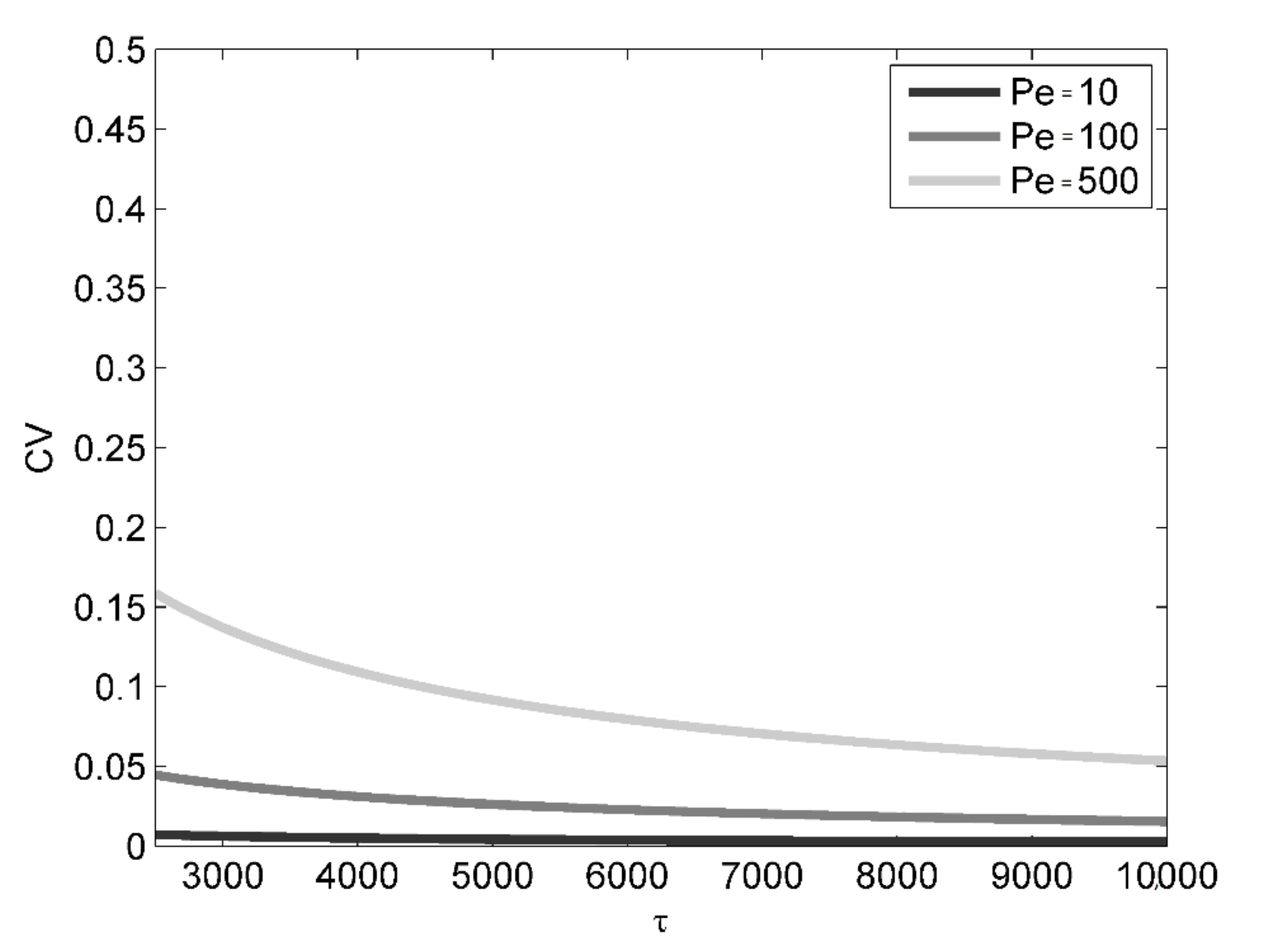
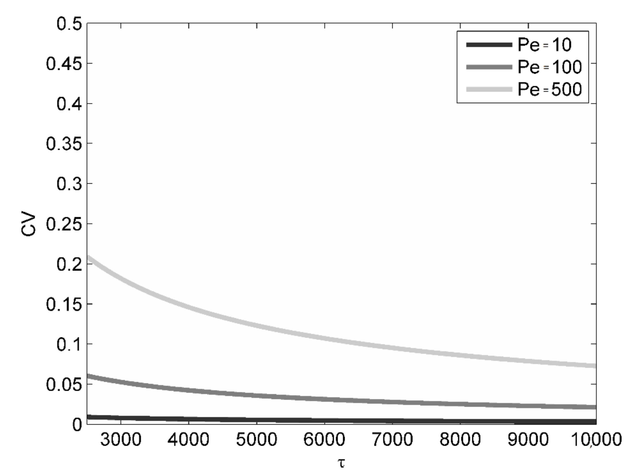
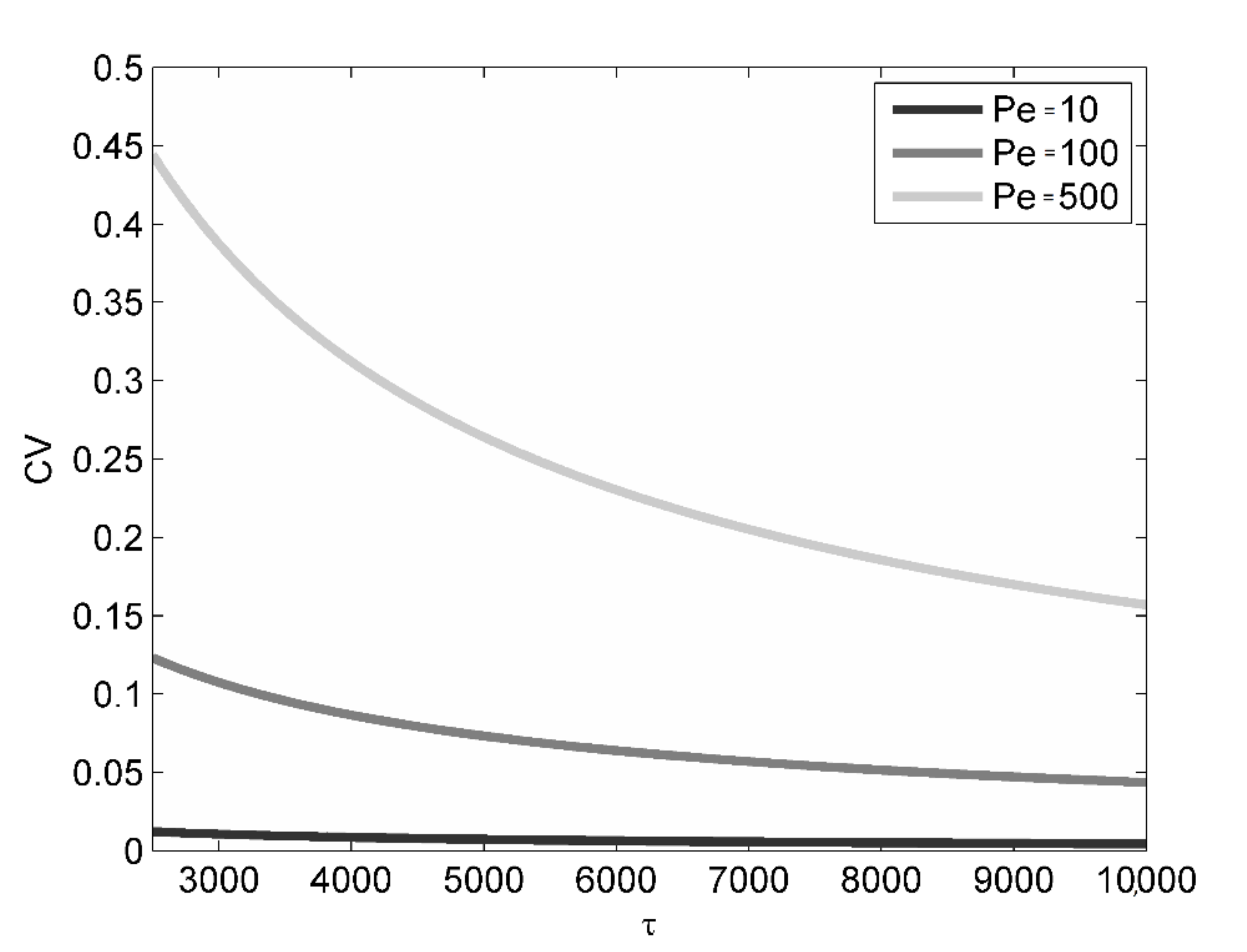
As one can see, except for Pe = 10 (a rather uncommon value of Péclet deriving from particularly intense local dispersion, slow flow and reduced log-conductivity integral scale), τω is characterized by very high values, even when one only requires that ω = 0.1 and the porous formation is mildly heterogeneous (). Consider, for example, τω for = 0.1 and Pe = 100: 1.727 × 10⁷. That means that, based on the large-time approximation for both X11 and S11, 1.727 × 10⁷ times the ratio is the time needed for a 90% reduction of the ratio S11/X11 (which still cannot be considered enough to represent really ergodic conditions). Note that IY is usually in the order of meters and V is frequently in the order of 10−6 to 10−5 meters/second. Therefore, one can conclude that there is practically no chance to achieve the theoretical ergodic domain where . The best one can do is therefore to evaluate CV and eventually to estimate as plus a suitable multiple of the standard deviation . By way of example, Figure 1, Figure 2 and Figure 3 respectively show, for = 1, 0.5 and 0.1, the large-time behavior of CV at a relatively short distance () from the expected moving centroid and peak of the Gaussian distribution (63) , when Pe = 10, 100 and 500.
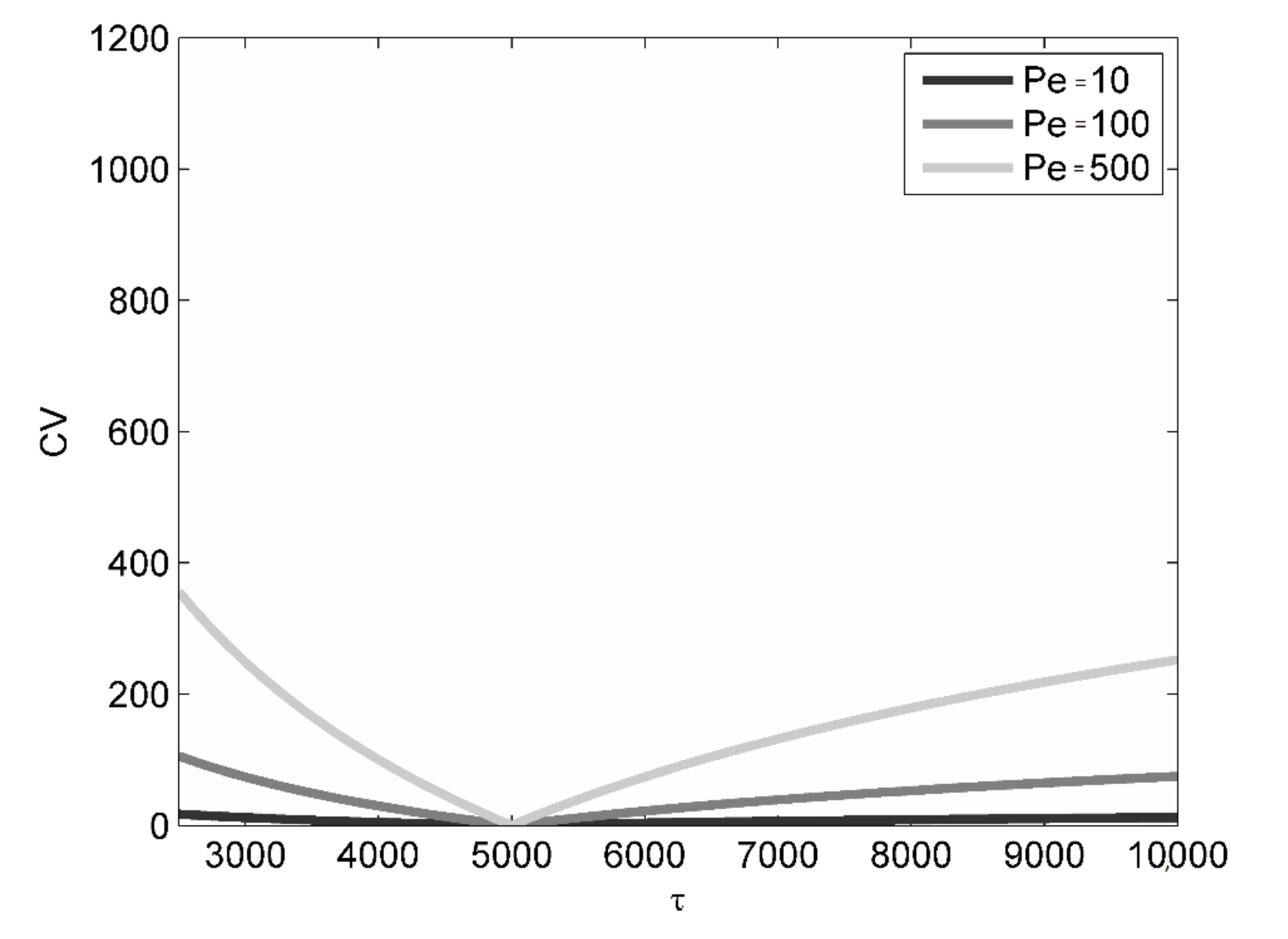
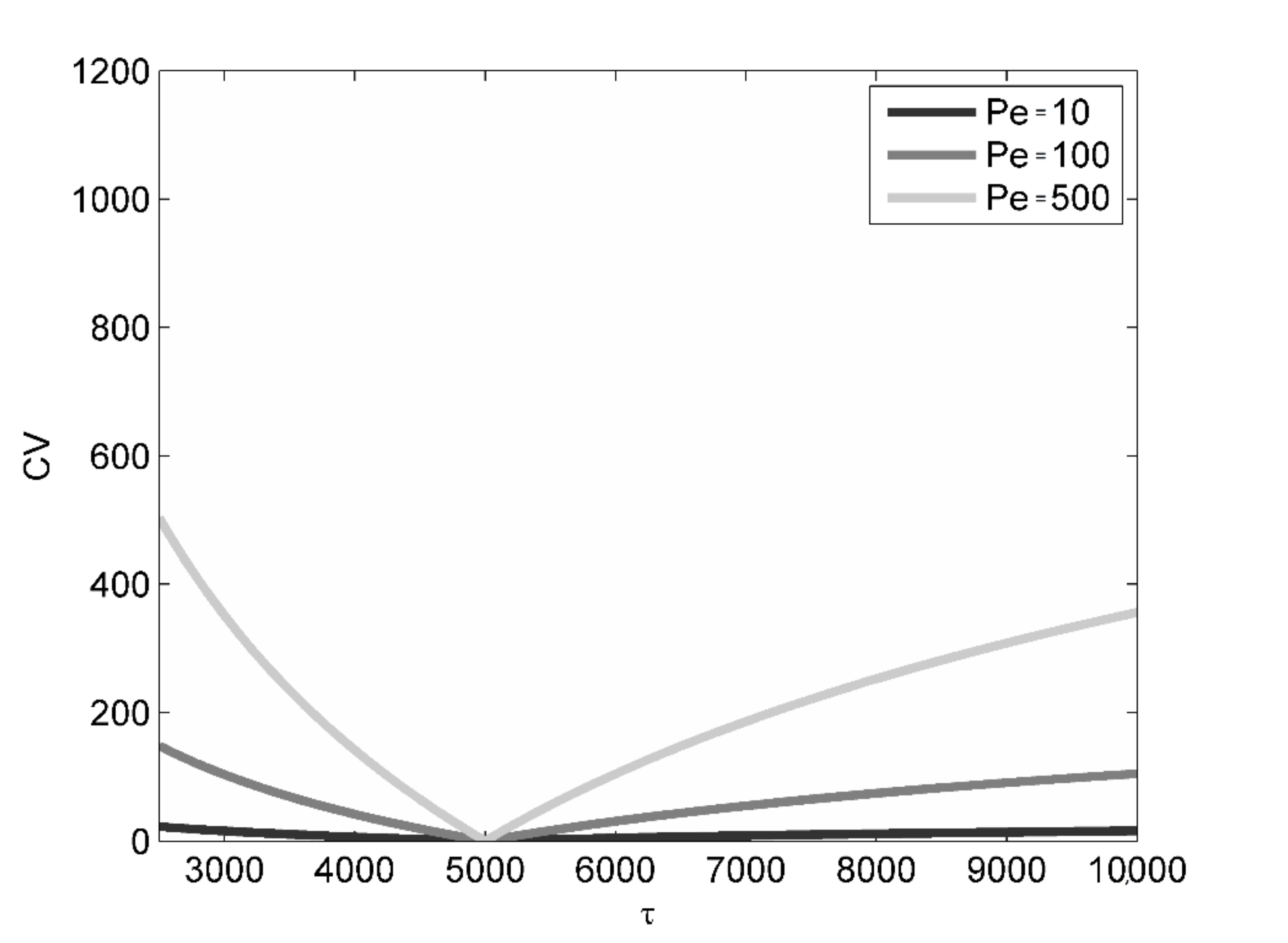
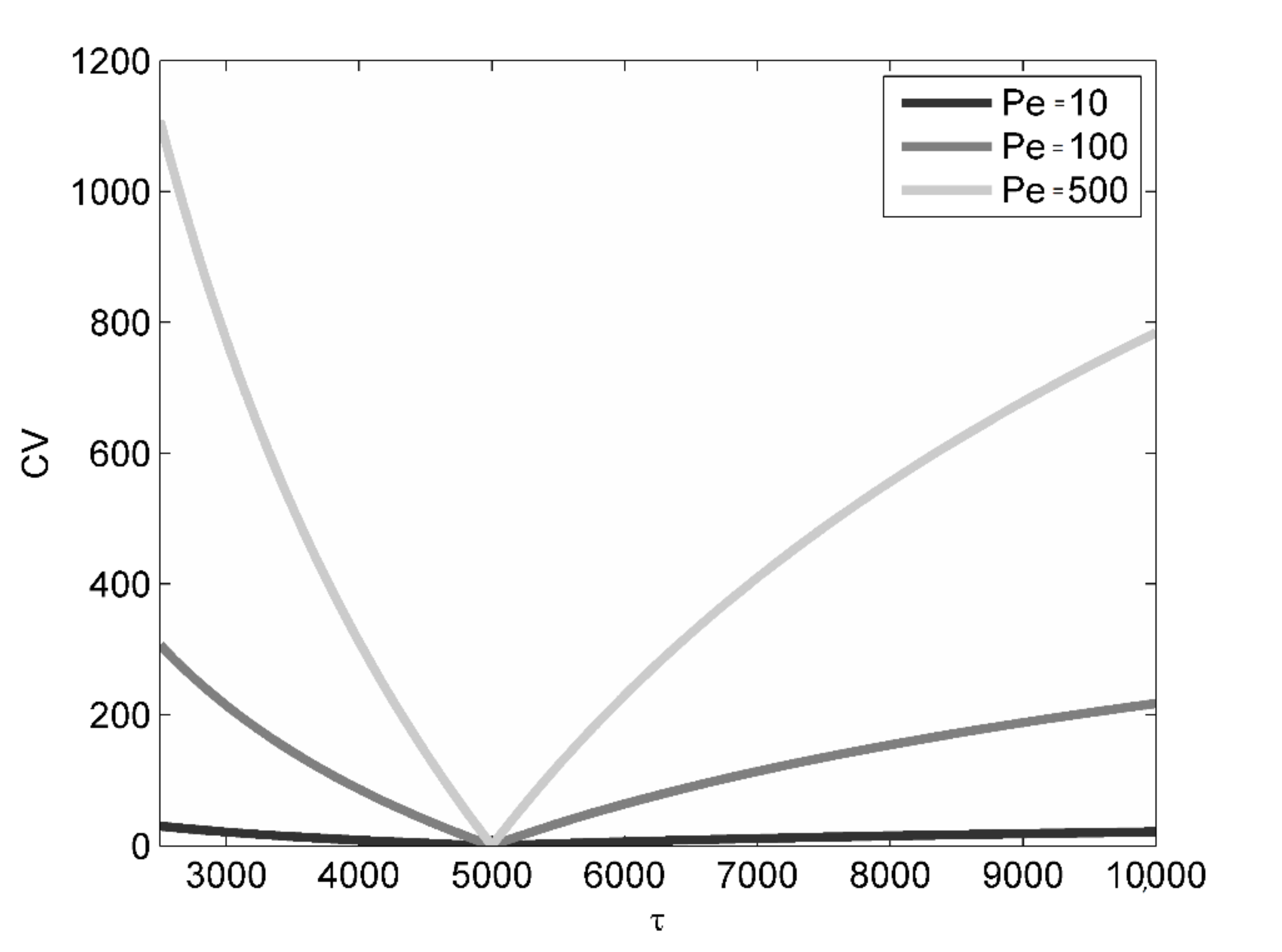
Note that based on the large-time concentration variance in Equation (47), the concentration coefficient of variation is zero at and increases with increasing distance from it. That means that the reliability of the concentration estimates deteriorates as their value decreases. As one can see, for given log-conductivity variance, CV is an increasing function of Pe. On the other hand, the three figures reveal that, whereas for diffusive or mildly advective regimes (Pe = 10 and Pe = 100), the level of heterogeneity expressed by only slightly affects CV, in the case of markedly advective regimes (Pe = 500), a more heterogeneous log-conductivity distribution () leads to faster CV reduction and, therefore, faster solute plume dilution. From a quantitative standpoint, Figure 3 (the worst scenario) says that a weakly heterogeneous formation in a markedly advective transport regime could require a travel distance of up to 10,000 integral scales to allow a standard deviation equal to 20% of the (relatively close to the peak) expected concentration value. For IY = 1 m, that would mean 10 km: that is, a travel distance hardly compatible with the typical dimensions of a hydraulically continuous aquifer and a residence time much larger than the typical times of technical interest. Finally, Figure 4, Figure 5 and Figure 6 show the large-time behavior of CV at a fixed point in space (x1 = 5000IY, x2 = 1IY, x3 = 1IY). Such a type of estimate (a sort of “Eulerian” CV) could be useful, as an example, when choosing the best location of agricultural or urban supply wells in the presence of possible upstream groundwater pollution sources.
As one can see, the concentration coefficient of variation experiences its minimum in correspondence of the centroid passage (τ = 5000). Overall, the values of CV at different times are always very high, except for very small Péclet. Obviously, it should be observed that the expected concentration quickly goes to zero far from the peak and the evaluation of the corresponding CV makes sense only if the toxicity threshold is very low. As for CV at a fixed distance from the moving centroid (the “Lagrangian” CV), we see that advective regimes are characterized by lower uncertainty when coupled with higher heterogeneity.
Thus, one can conclude that in transport processes that are dominated by advective mechanisms, the dissipative effect of local dispersion is exalted by flow field heterogeneity. This fully confirms what was postulated by [6] in terms of synergetic non-additive effect of advection and local dispersion in tracer dilution.
4. Discussion and Conclusions
The protection of groundwater resources, and the prediction of the time evolution of their accidental contamination, is one of the priorities in the field of environmental engineering. Many researchers in the last few decades have addressed theoretical, computational and experimental issues related to water flow and solute transport in heterogeneous porous formations. The importance of theoretical studies in this field (against the costs of extensive field surveys and the computational burden of realistic numerical simulations) resides in the possibility to design better targeted, smaller-scale interventions. Note that groundwater transport theories are typically applied to the saturated zone of aquifers. As a matter of fact, within the vadose zone, the lack of hydraulic continuity implies the absence of a longitudinal gradient. Fluid displacement only occurs along the vertical direction due to gravity and suction and usually ends (rather quickly) at the aquifer phreatic surface (or at the impervious boundary in the presence of semi-dry layers). One could say that infiltration across the unsaturated zone can eventually be viewed as the pre-initial condition for saturated transport. Moreover, the ubiquitous asymptotic character of the analytical formulations would not be consistent with the reduced temporal horizon of contaminant motion driven by gravity and capillary forces. Finally, the dangerousness of pollution events is mostly related to downstream propagation and its typical space–time uncertainty.
The present study makes use of a combined Eulerian–Lagrangian stochastic approach to evaluate centroid position uncertainty in the case of passive contaminant plumes originating from an instantaneous point source in statistically stationary and isotropic saturated porous formations, to assess the time needed for achieving the so-called ergodic conditions (which would allow for the evaluation of point concentrations based on the only Gaussian ensemble mean distribution), and to derive the large-time concentration coefficient of variation as a function of asymptotic macro-dispersion coefficients and centroid trajectory variances. The Eulerian part of the present formulation consists of making use of the advection–dispersion equation to derive the governing equation of the plume centroid second-order statistics and the equilibrium concentration variance approximation. The Lagrangian part consists of expressing the actual concentration distribution and, as a consequence, all its moments in terms of solute particle actual trajectories and related statistics. The results indicate that, even in mildly heterogeneous aquifers and mildly advective regimes, there is practically no chance to achieve the theoretical ergodic domain. Therefore, estimating the concentration coefficient of variation is essential for the prediction of point levels of exposure to toxic non-reactive substances accidentally carried out by groundwater, even at large times after contamination. The large-time coefficient of variation is zero at the moving centroid. At (short) fixed distances from it, CV is an increasing function of Péclet for given log-conductivity variance, and decays in time at a rate that is higher for more heterogeneous log-conductivity distributions. The concentration coefficient of variation evaluated at a fixed point in space experiences its minimum in correspondence of the centroid passage, but rapidly increases when the peak of the distribution moves away. Its values are always very large, except for unrealistically small Péclet. Obviously, it must be stressed that the expected concentration quickly goes to zero far from the peak of the distribution and the evaluation of the corresponding CV makes sense if the toxicity threshold is very low (which is the case for several contaminant chemicals). For both CV at a fixed distance from the moving centroid (the “Lagrangian” CV) and CV at a fixed point in space (the “Eulerian” CV), we see that the advective regimes (high Péclet) are characterized by lower uncertainty when coupled with higher heterogeneity. Thus, one can conclude that in the presence of relatively high Péclet numbers (transport processes dominated by advection), the dissipative effect of a relatively weak local dispersion is enhanced by large values of log-conductivity (and velocity) variance. As a matter of fact, large log-conductivity (and velocity) variance imply highly irregular concentration distributions and, as a consequence, large mass fluxes based on Fick’s law and more efficient homogenization processes. This fully confirms what was previously postulated by the author in terms of synergetic non-additive effect of advection and local dispersion in passive solute dilution. In the present study, it has also been shown that the ratio of the square root of the two-particle covariance (a sort of passive scalar micro-scale) to the average distance actually covered by the plume is proportional to the power −3/4 of the ratio of squared local dispersive length to squared log-conductivity integral scale. This is the same type of power law that governs the relationship between dimensionless turbulent Kolmogorov’s micro-scale and Reynolds number. As a matter of fact, momentum and mass transfer by chaotic flows are related by Reynolds’ analogy. The square root of the two-particle covariance can be considered as the tracer transport microscale and, therefore, the equivalent of Kolmogorov microscale η. The ratio of Kolmogorov microscale to the representative flow domain dimension L scales with the power −3/4 of Reynolds number. Reynolds number measures the relative magnitude of inertial and viscous effects, which can respectively be associated with the tendency of the flow to chaos and fast-decaying trajectories correlation, and to order and long-range trajectories correlation. As mass transport is an intrinsically unsteady process, the equivalent of L must be represented by the travel distance Vt, which measures the portion of the domain actually sampled by the solute body. Finally, the role of Reynolds number must be played by the ratio of two quantities that respectively symbolize uncorrelated and correlated particle displacements: the transverse area of the local dispersive spot about the average longitudinal trajectory (proportional to Dt) and the correlated area (proportional to IY2).
Finally, a further issue when dealing with real porous formations may be represented by their confinement by natural or artificial boundaries. In mathematical terms, confinement is equivalent to the exclusion of the contribution from the wave-number region around k = (0,0,0) (that is, the contribution from the largest scales of heterogeneity). As a consequence, in this case, log-conductivity and velocity could be considered as periodic functions to be expanded in Fourier series with a finite maximum period. With Fvii(k) indicating the discrete spectrum of the pair (v′i, v′i), one obtains at t→∞, from Equation (20) rewritten for the generic i:
the following asymptotic two-particle covariance:
Funding
This research received no external funding.
Conflicts of Interest
The author declares no conflict of interest.
References
- Bear, J. Dynamics of Fluids in Porous Media; Dover Publications Inc.: New York, NY, USA, 1972; 764p, ISBN 0486656756. [Google Scholar]
- Dagan, G. Flow and Transport in Porous Formations; Springer: New York, NY, USA, 1989; 465p, ISBN 3540510982. [Google Scholar]
- Rubin, Y. Applied Stochastic hydrogeology; Oxford University Press: London, UK, 2003; 416p, ISBN 9780198031543. [Google Scholar]
- Kapoor, V.; Gelhar, L.W. Transport in three-dimensionally heterogeneous aquifers: 1. Dynamics of concentration fluctuations. Water Resour. Res. 1994, 30, 1775–1788. [Google Scholar] [CrossRef]
- Kapoor, V.; Gelhar, L.W. Transport in three-dimensionally heterogeneous aquifers: 2. Predictions and observations of concentration fluctuations. Water Resour. Res. 1994, 30, 1789–1801. [Google Scholar] [CrossRef]
- Pannone, M.; Kitanidis, P.K. Large-time behavior of concentration variance and dilution in heterogeneous formations. Water Resour. Res. 1999, 35, 623–634. [Google Scholar] [CrossRef]
- Walters, P. An Introduction to Ergodic Theory; Springer: New York, NY, USA, 1982; 250p, ISBN 9780387951522. [Google Scholar]
- Pannone, M. Transient Hydrodynamic Dispersion in Rough Open Channels: Theoretical Analysis of Bed-Form Effects. J. Hydraul. Eng. ASCE 2010, 136, 155–164. [Google Scholar] [CrossRef]
- Pannone, M. Effect of nonlocal transverse mixing on river flows dispersion: A numerical study. Water Resour. Res. 2010, 46, W08534. [Google Scholar] [CrossRef]
- Pannone, M. Longitudinal Dispersion in River Flows Characterized by Random Large-Scale Bed Irregularities: First-Order Analytical Solution. J. Hydraul. Eng. ASCE 2012, 138, 400–411. [Google Scholar] [CrossRef]
- Pannone, M.; De Vincenzo, A.; Brancati, F. A Mathematical Model for the Flow Resistance and the Related Hydrodynamic Dispersion Induced by River Dunes. J. Appl. Math. 2013, 432610. [Google Scholar] [CrossRef] [Green Version]
- Pannone, M.; De Vincenzo, A. Stochastic numerical analysis of anomalous longitudinal dispersion and dilution in shallow decelerating stream flows. Stoch. Environ. Res. Risk Assess. 2015, 29, 2087–2100. [Google Scholar] [CrossRef]
- Pannone, M. An Analytical Model of Fickian and Non-Fickian Dispersion in Evolving-Scale Log-Conductivity Distributions. Water 2017, 9, 751. [Google Scholar] [CrossRef] [Green Version]
- Pannone, M. On the exact analytical solution for the spatial moments of the cross-sectional average concentration in open channel flows. Water Resour. Res. 2012, 48, W08511. [Google Scholar] [CrossRef]
- Pannone, M. Predictability of tracer dilution in large open channel flows: Analytical solution for the coefficient of variation of the depth-averaged concentration. Water Resour. Res. 2014, 50, 2617–2635. [Google Scholar] [CrossRef]
- Pannone, M.; Mirauda, D.; De Vincenzo, A.; Molino, B. Longitudinal Dispersion in Straight Open Channels: Anomalous Breakthrough Curves and First-Order Analytical Solution for the Depth-Averaged Concentration. Water 2018, 10, 478. [Google Scholar] [CrossRef] [Green Version]
- Kitanidis, P.K. Prediction by the method of moments of transport in heterogeneous formation. J. Hydrol. 1988, 102, 453–473. [Google Scholar] [CrossRef]
- Dagan, G. Transport in heterogeneous porous formations: Spatial moments, ergodicity, and effective dispersion. Water Resour. Res. 1990, 26, 1281–1290. [Google Scholar] [CrossRef]
- Pannone, M.; Kitanidis, P.K. Large-time spatial covariance of concentration of conservative solute and application to the Cape Cod tracer test. Transp. Porous Media 2001, 42, 109–132. [Google Scholar] [CrossRef]
- Tennekes, H.; Lumley, J.L. A First Course in Turbulence; MIT Press: Boston, MA, USA, 1972; 320p, ISBN 9780262200196. [Google Scholar]
- Gelhar, L.W.; Axness, C.L. Three-dimensional stochastic analysis of macrodispersion in aquifers. Water Resour. Res. 1983, 19, 161–180. [Google Scholar] [CrossRef]
- Mirauda, D.; De Vincenzo, A.; Pannone, M. Simplified entropic model for the evaluation of suspended load concentration. Water 2018, 10, 378. [Google Scholar] [CrossRef] [Green Version]
Publisher’s Note: MDPI stays neutral with regard to jurisdictional claims in published maps and institutional affiliations. |
Figure 1.
Concentration coefficient of variation at a given distance from the moving centroid . CV is the concentration coefficient of variation; τ is the dimensionless time.
Figure 1.
Concentration coefficient of variation at a given distance from the moving centroid . CV is the concentration coefficient of variation; τ is the dimensionless time.

Figure 2.
Concentration coefficient of variation at a given distance from the moving centroid . CV is the concentration coefficient of variation; τ is the dimensionless time.
Figure 2.
Concentration coefficient of variation at a given distance from the moving centroid . CV is the concentration coefficient of variation; τ is the dimensionless time.

Figure 3.
Concentration coefficient of variation at a given distance from the moving centroid . CV is the concentration coefficient of variation; τ is the dimensionless time.
Figure 3.
Concentration coefficient of variation at a given distance from the moving centroid . CV is the concentration coefficient of variation; τ is the dimensionless time.

Figure 4.
Concentration coefficient of variation at a fixed point in space . CV is the concentration coefficient of variation; τ is the dimensionless time.
Figure 4.
Concentration coefficient of variation at a fixed point in space . CV is the concentration coefficient of variation; τ is the dimensionless time.

Figure 5.
Concentration coefficient of variation at a fixed point in space . CV is the concentration coefficient of variation; τ is the dimensionless time.
Figure 5.
Concentration coefficient of variation at a fixed point in space . CV is the concentration coefficient of variation; τ is the dimensionless time.

Figure 6.
Concentration coefficient of variation at a fixed point in space . CV is the concentration coefficient of variation; τ is the dimensionless time.
Figure 6.
Concentration coefficient of variation at a fixed point in space . CV is the concentration coefficient of variation; τ is the dimensionless time.


Table 1.
Decay time of the ratio of two-particle to one-particle covariance. Pe: Péclet number; ω: decay percentage.
Table 1.
Decay time of the ratio of two-particle to one-particle covariance. Pe: Péclet number; ω: decay percentage.
| ω | Pe | 10 | 100 | 500 |
|---|---|---|---|---|
| 0.1 | 5.225 × 10³ | 1.727 × 10⁷ | 2.511 × 10⁹ | |
| 0.05 | 2.09 × 10⁴ | 6.909 × 10⁷ | 1.004 × 10¹⁰ | |
| 0.01 | 5.225 × 10⁵ | 1.727 × 10⁹ | 2.511 × 10¹¹ | |
Table 2.
Decay time of the ratio of two-particle to one-particle covariance. Pe: Péclet number; ω: decay percentage.
Table 2.
Decay time of the ratio of two-particle to one-particle covariance. Pe: Péclet number; ω: decay percentage.
| ω | Pe | 10 | 100 | 500 |
|---|---|---|---|---|
| 0.1 | 1.451 × 10⁴ | 2.009 × 10⁷ | 2.592 × 10⁹ | |
| 0.05 | 5.806 × 10⁴ | 8.035 × 10⁷ | 1.037 × 10¹⁰ | |
| 0.01 | 1.451 × 10⁶ | 2.009 × 10⁹ | 2.592 × 10¹¹ | |
© 2020 by the author. Licensee MDPI, Basel, Switzerland. This article is an open access article distributed under the terms and conditions of the Creative Commons Attribution (CC BY) license (http://creativecommons.org/licenses/by/4.0/).
Share and Cite
MDPI and ACS Style
Pannone, M. A Theoretical Study about Ergodicity Issues in Predicting Contaminant Plume Evolution in Aquifers. Water 2020, 12, 2929. https://doi.org/10.3390/w12102929
AMA Style
Pannone M. A Theoretical Study about Ergodicity Issues in Predicting Contaminant Plume Evolution in Aquifers. Water. 2020; 12(10):2929. https://doi.org/10.3390/w12102929
Chicago/Turabian StylePannone, Marilena. 2020. "A Theoretical Study about Ergodicity Issues in Predicting Contaminant Plume Evolution in Aquifers" Water 12, no. 10: 2929. https://doi.org/10.3390/w12102929
Note that from the first issue of 2016, this journal uses article numbers instead of page numbers. See further details here.