Comparisons of Performance Using Data Assimilation and Data Fusion Approaches in Acquiring Precipitable Water Vapor: A Case Study of a Western United States of America Area


Abstract
:1. Introduction
2. Research Area and Multi-Source Data
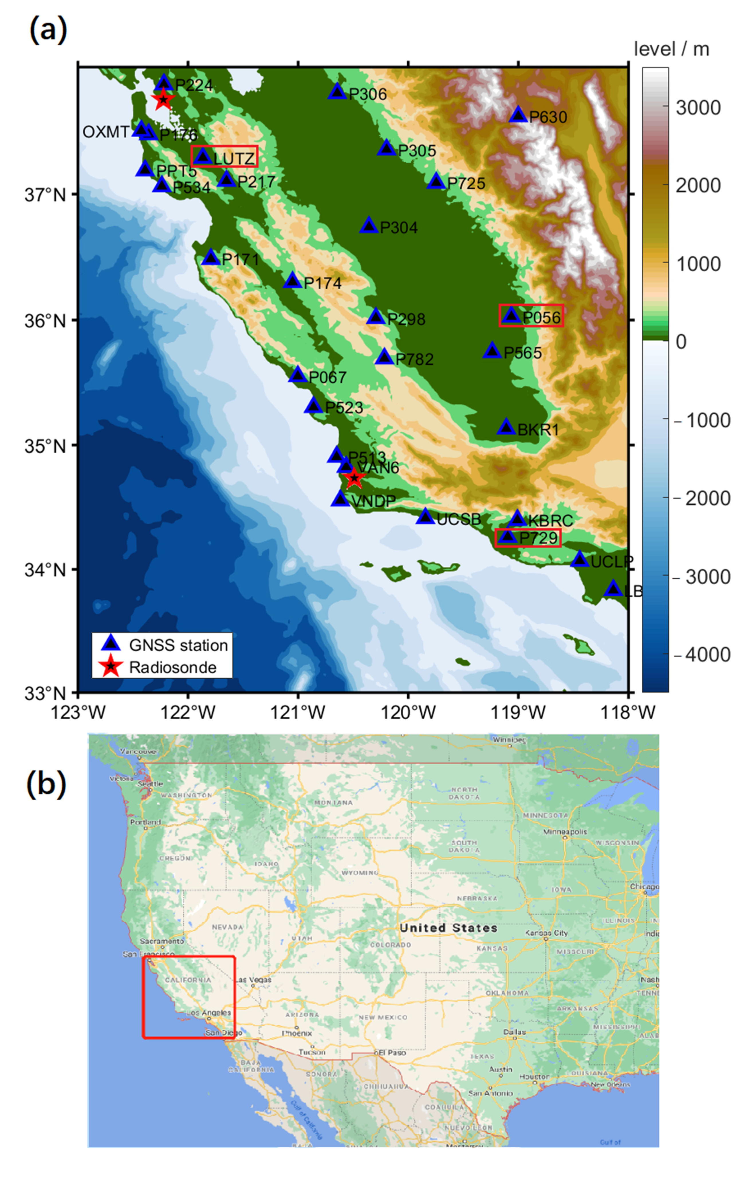
2.1. Research Area
2.2. Multi-Source Data
3. Method
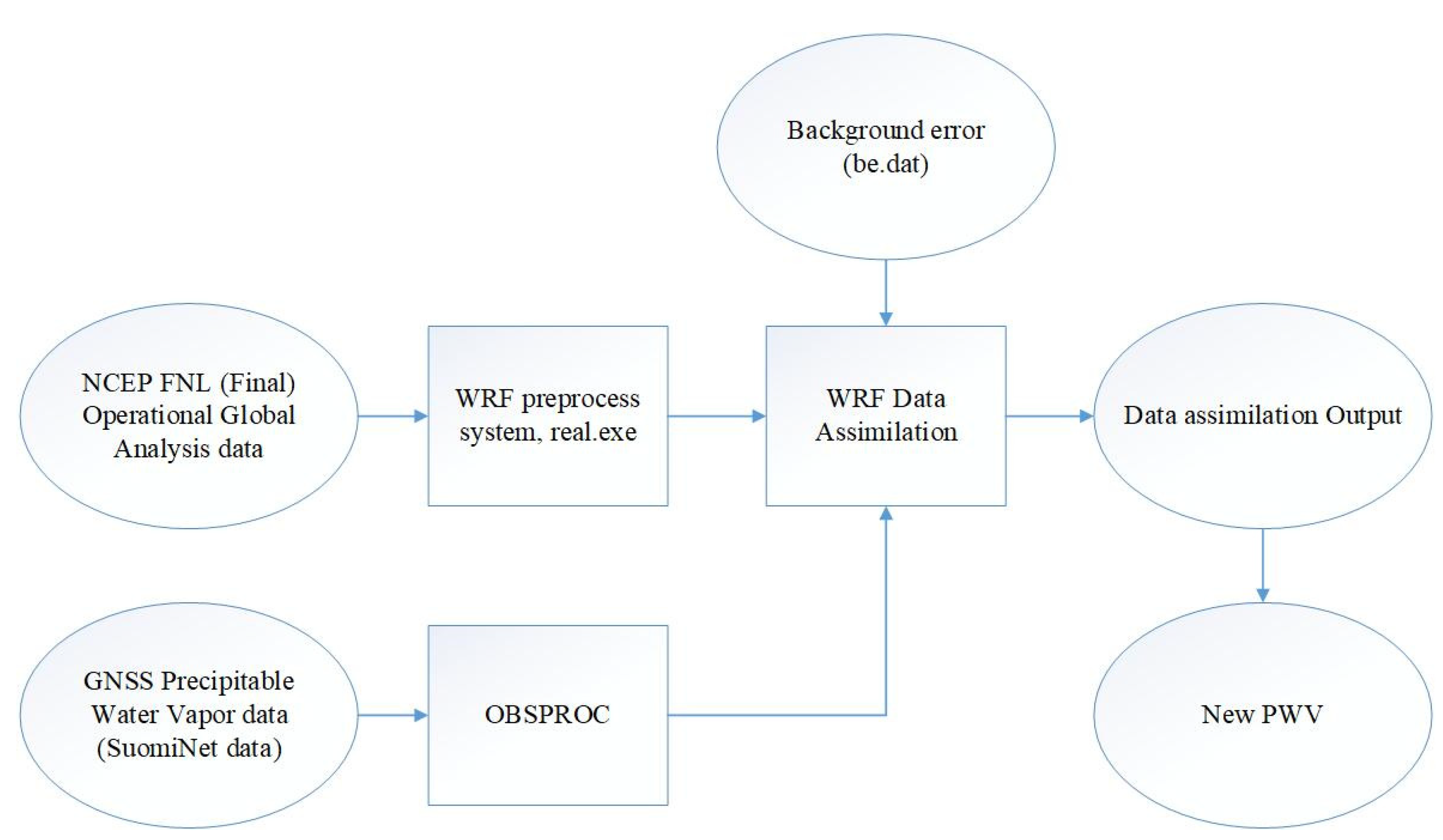
3.1. WRF Data Assimilation
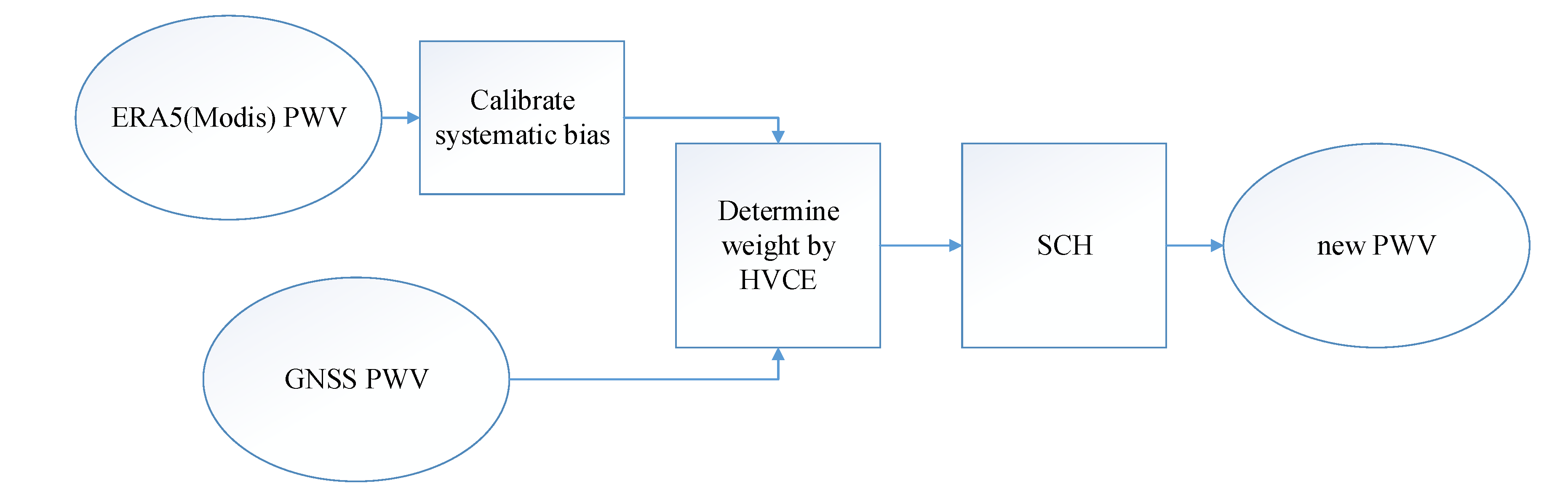
3.2. Data Fusion
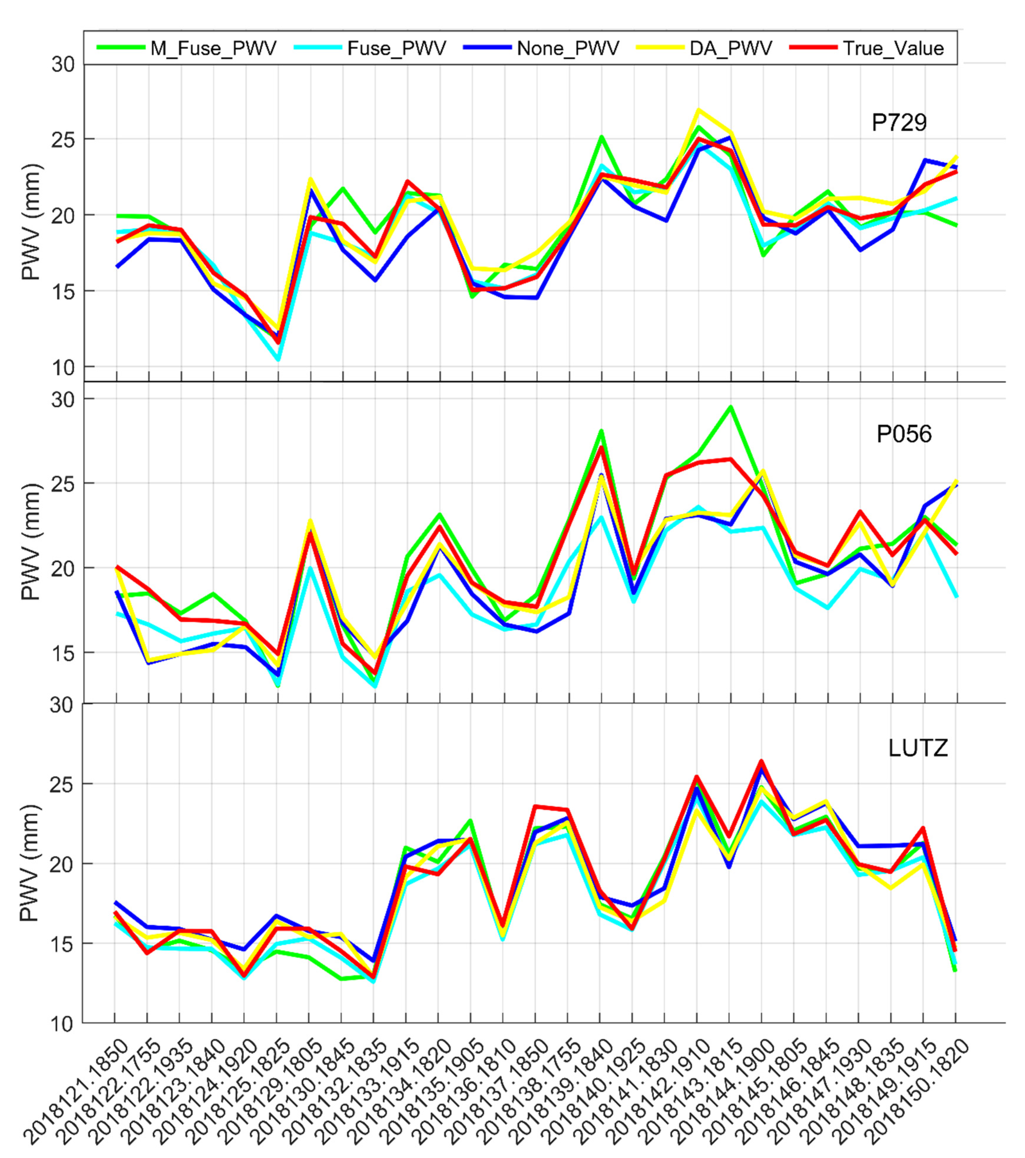
4. Results
5. Conclusions
Author Contributions
Funding
Conflicts of Interest
Abbreviations
| Abbreviations | Full Name |
| DA | Data assimilation |
| DOY | Days of year |
| ECWMF | European Centre for Medium-Range Weather Forecasts |
| ERA5 | ECWMF Reanalysis 5 |
| FNL | Final |
| GDAS | Global Data Assimilation System |
| GNSS | Global Navigation Satellite System |
| HVCE | Helmert variance component estimation |
| IGRA | Integrated Global Radiosonde Archive |
| InSAR | Interferometric synthetic aperture radar |
| IR | Infrared |
| JMA | Japan Meteorological Agency |
| MODIS | Moderate-resolution imaging spectroradiometer |
| MMM | Mesoscale and Microscale Meteorology |
| NCAR | National Center for Atmospheric Research |
| NCEP | National Centers for Environmental Prediction |
| NCL | NCAR Command Language |
| NIR | Near infrared |
| NWP | Numerical weather prediction |
| PBL | Planetary boundary layer |
| PWV | Precipitable water vapor |
| RH | Relative humidity |
| RMS | Root mean square |
| SCH | Spherical cap harmonic |
| SRM | Singapore Regional Model |
| SRMC | Singapore Regional Model Coarse |
| STD | Standard deviation |
| STRMDEM | Shuttle Radar Topography Mission Digital Elevation Model |
| WPS | WRF preprocess system |
| WRF | Weather Research and Forecasting |
| ZHD | Zenith hydrostatic delay |
| ZTD | Zenith total delay |
| ZWD | Zenith wet delay |
References
- American Meteorological Society (AMS). Glossary of Meteorology, 2nd ed.; American Meteorological Society (AMS): Boston, MA, USA, 2000. [Google Scholar]
- Zhang, B.; Yao, Y.; Xin, L.; Xu, X. Precipitable water vapor fusion: An approach based on spherical cap harmonic analysis and Helmert variance component estimation. J. Geod. 2019, 93, 2605–2620. [Google Scholar] [CrossRef]
- Sharifi, M.A.; Azadi, M.; Khaniani, A.S. Numerical simulation of rainfall with assimilation of conventional and GPS observations over north of Iran. Ann. Geophys. 2016, 59, 0322. [Google Scholar]
- Mateus, P.; Tomé, R.; Nico, G.; Catalão, J. Three-Dimensional Variational Assimilation of InSAR PWV Using the WRFDA Model. IEEE Trans. Geosci. Remote Sens. 2016, 54, 7323–7330. [Google Scholar] [CrossRef]
- Saito, K.; Shoji, Y.; Origuchi, S.; Duc, L. GPS PWV assimilation with the JMA nonhydrostatic 4DVAR and cloud resolving ensemble forecast for the 2008 August Tokyo metropolitan area local heavy rainfalls. In Data Assimilation for Atmospheric, Oceanic and Hydrologic Applications (Vol. III); Springer: Cham, Switzerland, 2017; pp. 383–404. [Google Scholar]
- Pacione, R.; Sciarretta, C.; Faccani, C.; Ferretti, R.; Vespe, F. GPS PW assimilation into MM5 with the nudging technique. Phys. Chem. Earth Part A 2001, 26, 481–485. [Google Scholar] [CrossRef]
- Faccani, C.; Ferretti, R.; Pacione, R.; Paolucci, T.; Vespe, F.; Cucurull, L. Impact of a high density GPS network on the operational forecast. Adv. Geosci. 2005, 2, 73–79. [Google Scholar] [CrossRef] [Green Version]
- Bennitt, G.V.; Jupp, A. Operational Assimilation of GPS Zenith Total Delay Observations into the Met Office Numerical Weather Prediction Models. Mon. Weather Rev. 2012, 140, 2706–2719. [Google Scholar] [CrossRef]
- Lindskog, M.; Ridal, M.; Thorsteinsson, S.; Ning, T. Data assimilation of GNSS zenith total delays from a Nordic processing centre. Atmos. Chem. Phys. 2017, 17, 13983–13998. [Google Scholar] [CrossRef] [Green Version]
- Wang, X.; Babovic, V.; Li, X. Application of spatial-temporal error correction in updating hydrodynamic model. J. Hydro-Environ. Res. 2017, 16, 45–57. [Google Scholar] [CrossRef]
- Wang, X.; Zhang, J.; Babovic, V. Improving real-time forecasting of water quality indicators with combination of process-based models and data assimilation technique. Ecol. Indic. 2016, 66, 428–439. [Google Scholar] [CrossRef]
- Karri, R.; Vladan, B. Enhanced predictions of tides and surges through data assimilation. Int. J. Eng. 2017, 30, 23–29. [Google Scholar]
- Li, Z. Production of regional 1 km x 1 km water vapor fields through the integration of GPS and MODIS data. Am. J. Public Hyg. 2004, 19, 1443–1450. [Google Scholar]
- Alshawaf, F.; Hinz, S.; Mayer, M.; Meyer, F.J. Constructing accurate maps of atmospheric water vapor by combining interferometric synthetic aperture radar and GNSS observations. J. Geophys. Res. 2015, 120, 1391–1403. [Google Scholar] [CrossRef]
- Babovic, V.; Caňizares, R.; Jensen, H.R.; Klinting, A. Neural networks as routine for error updating of numerical models. J. Hydraul. Eng. 2001, 127, 181–193. [Google Scholar] [CrossRef]
- Sun, Y.; Babovic, V.; Chan, E.S. Multi-step-ahead model error prediction using time-delay neural networks combined with chaos theory. J. Hydrol. 2010, 395, 109–116. [Google Scholar] [CrossRef]
- Reuter, H.I.; Nelson, A.; Jarvis, A. An evaluation of void-filling interpolation methods for SRTM data. Int. J. Geogr. Inf. Sci. 2007, 21, 983–1008. [Google Scholar] [CrossRef]
- Jarvis, A.; Reuter, H.I.; Nelson, A.; Guevara, E. Hole-Filled Seamless SRTM Data V4, International Centre for Tropical Agriculture (CIAT). 2008. Available online: http://srtm.csi.cgiar.org (accessed on 9 October 2019).
- Ware, R.H.; Fulker, D.W.; Stein, S.A.; Anderson, D.N.; Avery, S.K.; Clark, R.D.; Droegemeier, K.K.; Kuettner, J.P.; Minster, J.B.; Sorooshian, S. SuomiNet: A real-time national GPS network for atmospheric research and education. Bull. Am. Meteorol. Soc. 2000, 81, 677–694. [Google Scholar] [CrossRef] [Green Version]
- UCAR/NCAR/CISL/VETS: The NCAR Command Language (NCL, Version 6.1.2), UCAR/NCAR/CISL/VETS, Boulder, Colorado, 2013. Available online: http://www.ncl.ucar.edu/ (accessed on 9 October 2019).
- Yao, Y.; Zhang, B.; Xu, C.; Yan, F. Improved one/multi-parameter models that consider seasonal and geographic variations for estimating weighted mean temperature in ground-based GPS meteorology. J. Geod. 2014, 88, 273–282. [Google Scholar] [CrossRef]
- Vedel, H.; Huang, X.Y.; Haase, J.; Ge, M.; Calais, E. Impact of GPS zenith tropospheric delay data on precipitation forecasts in Mediterranean France and Spain. Geophys. Res. Lett. 2004, 31, L02102. [Google Scholar] [CrossRef] [Green Version]
- Xiong, Z.; Zhang, B.; Yao, Y. Comparisons between the WRF data assimilation and the GNSS tomography technique in retrieving 3-D wet refractivity fields in Hong Kong. Ann. Geophys. 2019, 37, 25–36. [Google Scholar] [CrossRef] [Green Version]
- Chen, S.H.; Zhao, Z.; Haase, J.S.; Chen, A.; Vandenberghe, F. A Study of the Characteristics and Assimilation of Retrieved MODIS Total Precipitable Water Data in Severe Weather Simulations. Mon. Weather Rev. 2007, 136, 9052–9062. [Google Scholar] [CrossRef] [Green Version]
- Prasad, A.K.; Singh, R.P. Validation of MODIS Terra, AIRS, NCEP/DOE AMIP-II Reanalysis-2, and AERONET Sun photometer derived integrated precipitable water vapor using ground-based GPS receivers over India. J. Geophys. Res. Atmos. 2009, 114, D05107. [Google Scholar] [CrossRef] [Green Version]
- Chang, L.; Gao, G.; Jin, S.; He, X.; Xiao, R.; Guo, L. Calibration and Evaluation of Precipitable Water Vapor from MODIS Infrared Observations at Night. IEEE Trans. Geosci. Remote Sens. 2014, 53, 2612–2620. [Google Scholar] [CrossRef]
- Haines, G.V. Spherical cap harmonic analysis. J. Geophys. Res. Solid Earth 1985, 90, 2583–2591. [Google Scholar] [CrossRef]
- Koch, K.; Kusche, J. Regularization of geopotential determination from satellite data by variance components. J. Geod. 2002, 76, 259–268. [Google Scholar] [CrossRef]
- Xu, P.; Shen, Y.; Fukuda, Y.; Liu, Y. Variance Component Estimation in Linear Inverse Ill-posed Models. J. Geod. 2006, 80, 69–81. [Google Scholar] [CrossRef]


| Resolution (m) | 5000 | 7500 | 10,000 | 12,500 |
|---|---|---|---|---|
| Bias | 1.14 | 1.19 | 1.20 | 1.15 |
| STD | 1.57 | 1.55 | 1.57 | 1.60 |
| RMS | 1.91 | 1.93 | 1.94 | 1.94 |
| Resolution (m) | 5000 | 7500 | 10,000 | 12,500 | |
|---|---|---|---|---|---|
| T (K) | Bias | −0.08 | −0.08 | −0.08 | −0.09 |
| STD | 1.74 | 1.73 | 1.73 | 1.72 | |
| RMS | 1.74 | 1.73 | 1.73 | 1.73 | |
| P (hPa) | Bias | 0.56 | 0.57 | 0.56 | 0.55 |
| STD | 0.59 | 0.60 | 0.63 | 0.60 | |
| RMS | 0.81 | 0.83 | 0.84 | 0.82 | |
| RH (%) | Bias | 1.82 | 1.81 | 1.83 | 1.80 |
| STD | 13.38 | 13.34 | 13.36 | 13.34 | |
| RMS | 13.49 | 13.45 | 13.47 | 13.46 |
| None_PWV | DA_PWV | |||||||
|---|---|---|---|---|---|---|---|---|
| P729 | P056 | LUTZ | All | P729 | P056 | LUTZ | All | |
| Bias | −0.66 | −1.21 | 0.24 | −0.54 | 0.43 | −0.77 | −0.39 | −0.25 |
| STD | 1.20 | 1.95 | 1.11 | 1.57 | 0.95 | 1.87 | 1.16 | 1.46 |
| RMS | 1.35 | 2.27 | 1.12 | 1.65 | 1.02 | 1.99 | 1.21 | 1.47 |
| Fuse_PWV | M_Fuse_PWV | |||||||
| P729 | P056 | LUTZ | All | P729 | P056 | LUTZ | All | |
| Bias | −0.46 | −1.99 | −0.81 | −1.09 | 0.09 | 0.11 | −0.41 | −0.07 |
| STD | 0.71 | 1.04 | 0.75 | 1.06 | 1.38 | 1.16 | 0.88 | 1.17 |
| RMS | 0.84 | 2.23 | 1.09 | 1.52 | 1.36 | 1.15 | 0.96 | 1.17 |
Publisher’s Note: MDPI stays neutral with regard to jurisdictional claims in published maps and institutional affiliations. |
© 2020 by the authors. Licensee MDPI, Basel, Switzerland. This article is an open access article distributed under the terms and conditions of the Creative Commons Attribution (CC BY) license (http://creativecommons.org/licenses/by/4.0/).
Share and Cite
Xiong, Z.; Sang, J.; Sun, X.; Zhang, B.; Li, J. Comparisons of Performance Using Data Assimilation and Data Fusion Approaches in Acquiring Precipitable Water Vapor: A Case Study of a Western United States of America Area. Water 2020, 12, 2943. https://doi.org/10.3390/w12102943
Xiong Z, Sang J, Sun X, Zhang B, Li J. Comparisons of Performance Using Data Assimilation and Data Fusion Approaches in Acquiring Precipitable Water Vapor: A Case Study of a Western United States of America Area. Water. 2020; 12(10):2943. https://doi.org/10.3390/w12102943
Chicago/Turabian StyleXiong, Zhaohui, Jizhang Sang, Xiaogong Sun, Bao Zhang, and Junyu Li. 2020. "Comparisons of Performance Using Data Assimilation and Data Fusion Approaches in Acquiring Precipitable Water Vapor: A Case Study of a Western United States of America Area" Water 12, no. 10: 2943. https://doi.org/10.3390/w12102943